Author:
(1) David Staines.
Table of Links
4 Calvo Framework and 4.1 Household’s Problem
4.3 Household Equilibrium Conditions
4.5 Nominal Equilibrium Conditions
4.6 Real Equilibrium Conditions and 4.7 Shocks
5.2 Persistence and Policy Puzzles
6 Stochastic Equilibrium and 6.1 Ergodic Theory and Random Dynamical Systems
7 General Linearized Phillips Curve
8 Existence Results and 8.1 Main Results
9.2 Algebraic Aspects (I) Singularities and Covers
9.3 Algebraic Aspects (II) Homology
9.4 Algebraic Aspects (III) Schemes
9.5 Wider Economic Interpretations
10 Econometric and Theoretical Implications and 10.1 Identification and Trade-offs
10.4 Microeconomic Interpretation
Appendices
A Proof of Theorem 2 and A.1 Proof of Part (i)
B Proofs from Section 4 and B.1 Individual Product Demand (4.2)
B.2 Flexible Price Equilibrium and ZINSS (4.4)
B.4 Cost Minimization (4.6) and (10.4)
C Proofs from Section 5, and C.1 Puzzles, Policy and Persistence
D Stochastic Equilibrium and D.1 Non-Stochastic Equilibrium
D.2 Profits and Long-Run Growth
E Slopes and Eigenvalues and E.1 Slope Coefficients
E.4 Rouche’s Theorem Conditions
F Abstract Algebra and F.1 Homology Groups
F.4 Marginal Costs and Inflation
G Further Keynesian Models and G.1 Taylor Pricing
G.3 Unconventional Policy Settings
H Empirical Robustness and H.1 Parameter Selection
I Additional Evidence and I.1 Other Structural Parameters
I.3 Trend Inflation Volatility
B.2 Flexible Price Equilibrium and ZINSS (4.4)
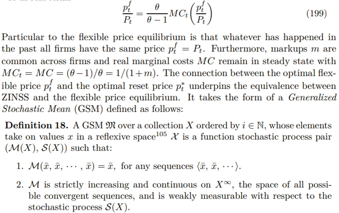
This subsection clarifies remarks concerning the relationship between the optimal reset price and the flexible price equilibrium, including their coincidence when there is zero inflation. To achieve this I introduce a little mathematical machinery, that I understand to be original. Under monopolistic competition, I find that the optimal price is a mark-up m = 1/(θ − 1) over marginal costs, so in real terms

It is worth briefly motivating this definition. Continuity and increasing requirements support the idea of the mean as an average and rule out alternative measures of location, such as median and mode.[106] The function space assumption allows us to include expectations of future variables, as part of our average ensemble. It is this averaging property that underpins ergodicity and mixing in the model.

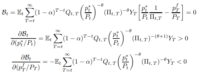
Proof. Weak measurability comes from the structure of the optimization problem. Monotonicity and continuity follow from the following implicit function argument, where the left-hand side is (27), combined with (199) and the gross inflation definition (23) on the right-hand side

Hence

Corollary 3. ZINSS is equivalent to a flexible price equilibrium.

Therefore uniquely at ZINSS the reset price constraint is not binding. This confirms the breakdown of nominal rigidity as the root cause of the bifurcation. The other weighted measures feature expectations of non-linear terms and are therefore not amenable to our definition.
Remark 36. These results carry over easily to alternative settings with finite price lives. This includes Taylor pricing and models where the price spell is truncated, such as Wolman [1999] and Dixon and Le Bihan [2012].
The final result justifies a comment in Footnote 25 in Section 4.4. It explains the distinction between the reset price and the flexible price. Moreover, it presages the idea of a limiting fringe of flexible price firms, used in Section 9.5 to make distinctions between real and nominal rigidity.
Proposition 28. The magnitude of the change in the reset price weakly exceeds the change in the price of a firm that always had flexible prices, with equality only when neither price changes.
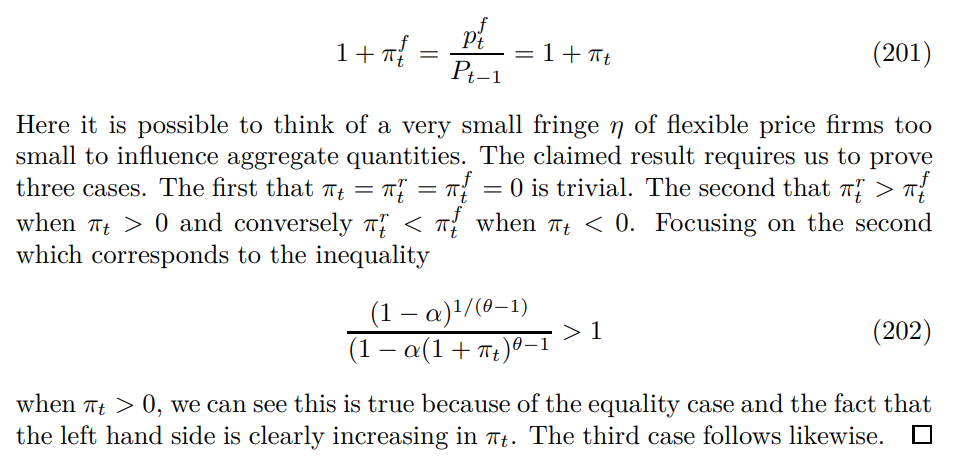
Proof. Since price re-setters are randomly assigned here, by a standard law of large numbers argument, the reset price inflation is given by

A flexible price firm will always set its price equal to the general price level

(202) corresponds to Proposition 1, the economic idea that the relative price of the re-setter is increasing in inflation. Intuitively, with rigid prices to generate inflation or deflation, re-setters have to adjust more aggressively than in the flexible price world, in order to make up for the portion of the price level that does not change. This is why we cannot naively compare observed price changes with a classical benchmark to obtain the spillover from rigid prices to flexible prices.
This paper is available on arxiv under CC 4.0 license.
[105] A reflexive space has the property that the set of possible ensemble averages and the set of possible realizations coincide.
[106] Consult Bullen [2003] for a review of mean concepts and their inequalities.

