Author:
(1) David Staines.
Table of Links
4 Calvo Framework and 4.1 Household’s Problem
4.3 Household Equilibrium Conditions
4.5 Nominal Equilibrium Conditions
4.6 Real Equilibrium Conditions and 4.7 Shocks
5.2 Persistence and Policy Puzzles
6 Stochastic Equilibrium and 6.1 Ergodic Theory and Random Dynamical Systems
7 General Linearized Phillips Curve
8 Existence Results and 8.1 Main Results
9.2 Algebraic Aspects (I) Singularities and Covers
9.3 Algebraic Aspects (II) Homology
9.4 Algebraic Aspects (III) Schemes
9.5 Wider Economic Interpretations
10 Econometric and Theoretical Implications and 10.1 Identification and Trade-offs
10.4 Microeconomic Interpretation
Appendices
A Proof of Theorem 2 and A.1 Proof of Part (i)
B Proofs from Section 4 and B.1 Individual Product Demand (4.2)
B.2 Flexible Price Equilibrium and ZINSS (4.4)
B.4 Cost Minimization (4.6) and (10.4)
C Proofs from Section 5, and C.1 Puzzles, Policy and Persistence
D Stochastic Equilibrium and D.1 Non-Stochastic Equilibrium
D.2 Profits and Long-Run Growth
E Slopes and Eigenvalues and E.1 Slope Coefficients
E.4 Rouche’s Theorem Conditions
F Abstract Algebra and F.1 Homology Groups
F.4 Marginal Costs and Inflation
G Further Keynesian Models and G.1 Taylor Pricing
G.3 Unconventional Policy Settings
H Empirical Robustness and H.1 Parameter Selection
I Additional Evidence and I.1 Other Structural Parameters
I.3 Trend Inflation Volatility
H.2 Phillips Curve
This subsection is split in two. The first part covers two alternative benchmarks. The second studies robustness at the standard settings and draws a comparison with the existing solution and empirics. Most emphasis is placed on the output slope coefficient in relation to macroeconometric estimates.
H.2.1 Alternative Cases.

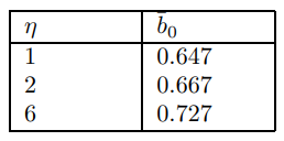
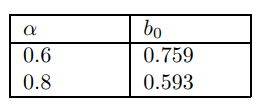
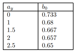
Note that in the later case only the lagged inflation coefficient changes substantially from the text. Movements in the other coefficients are much smaller. It is interesting to look at how the cut-off value of the lag varies as the various parameters are varied. Information on the other coefficients in these cases comes in the next part. Note that the cut-off is always less than unity. [135] This reflects the fact that inflation has to be stationary. The following triptych of tables alter parameters one at a time, keeping the others at the standard setting.

H.2.2 Benchmark Parametization
In this subsection, I study changes in the Phillips curve slope coefficients when structural parameters are varied, over the ranges discussed in the previous section. I then perform a similar exercise for the existing solution. The difference remains stark. This should be a spur for future rigorous econometric research.

The lagged inflation coefficient seems to be almost invariant to changes in the supply side, which is encouraging. The lead is also relatively unresponsive. This is encouraging from a Keynesian perspective. I anticipate the model will soon be augmented with additional frictions to better model the propagation of monetary shocks to labor and capital markets. I anticipate the model will soon be augmented with additional frictions to better model the propagation of monetary shocks to labor and capital markets. This will rest upon the robust foundation of our new understanding of inflation determination embodied in these coefficients.


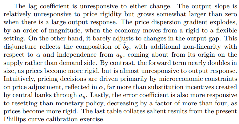

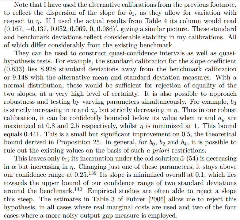
Overall, this part has provided a strong body of suggestive evidence that the new approximation provides a better fit than the existing coefficient by coefficient. Moreover, the stability of the critical slope coefficients, in response to plausible structural parameter uncertainty, is a showcase for robustness in macroeconomics. This exercise has surely been a useful prelude to future rigorous econometric investigation.
This paper is available on arxiv under CC 4.0 license.
[135] To see why this is true note that I can express the cut off as


[139] This occurs when I adjust α to 0.8, when η = 1 it is higher at 0.333.
[140] This conclusion is robust to any of the three deviation measures.

