Andrea Renzetti, Department of Economics, Alma Mater Studiorium Universit`a di Bologna, Piazza Scaravilli 2, 40126 Bologna, Italy.
Table of Links
Forecasting with the TC-TVP-VAR
Response analysis at the ZLB with the TC-TVP-VAR
4 Response analysis at the ZLB with the TC-TVP-VAR
TVP-VAR are extensively used in applied research not only to make forecasts, but also to infer changes in the response of the economy to macroeconomic shocks. In this section, I show that the proposed shrinkage prior can be useful also to enhance inference on the impulse response functions estimated from a TVP-VAR. Recent studies in empirical macroeconomics have used
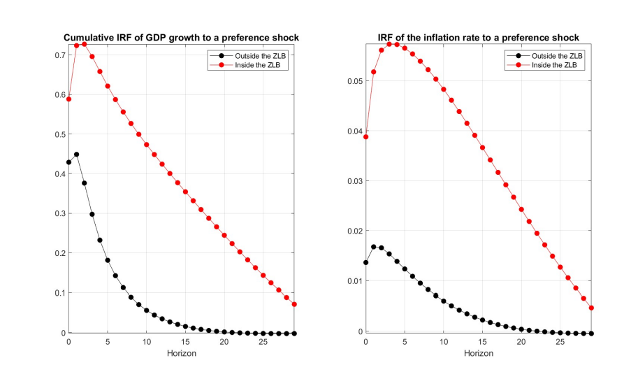
TVP-VARs to assess whether the US economy’s performance was affected by a binding ZLB constraint (Debortoli et al. 2019; Benati et al. 2023). As a matter of fact, according to a standard New-Keynesian model, the economy is expected to exhibit different responses when the ZLB constraint is in effect. For example, the model predicts a distinct response of output and inflation following both demand and supply shocks when the conventional stabilizing monetary policy response to aggregate shocks is constrained as a consequence of the Federal Funds Rate hitting the ZLB. Figure 3 makes this point, by showing the responses to a pure demand shock (preference shock) in the Smets et al. (2007) model version considered in Del Negro et al. (2015).[24] As expected, when monetary policy is constrained by the policy rate hitting the zero lower bound, the response of both output and inflation to the preference shock is magnified on impact and the effect of the shock dies down much more slowly over time.
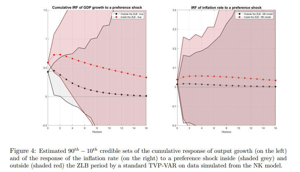
Despite the sharp difference in the propagation of the shocks in the economy inside and outside the zero lower bound period foreseen by a standard NK model, empirical evidences investigating this issue are mixed and many studies do not find substantial evidence supporting a different response of the US economy during the zero lower bound period. For example, Debortoli et al. (2019), support the irrelevance hypothesis i.e. the hypothesis that the economy’s performance has not been affected by a binding ZLB constraint, embracing the view that unconventional monetary policy have been effective at getting around the zero lower bound (ZLB) constraint. Benati et al. (2023) recently showed that, given the short length of the zero-lowerbound period, inference based on a standard TVP-VAR where the time varying parameters are regarded as slow moving stochastic processes, doesn’t allow to capture the changing relationship among the macroeconomic variables during the ZLB period predicted by the New Keynesian model. In what follows, based on a simulation study, I also find that a standard TVP-VAR struggles to detect the change in the responses of the economy in the ZLB period generated by a NK model. I show that the TC-TVP-VAR can in principle be used to solve this inferential issue and therefore to recover the distinct response of the economy during the zero lower bound period.
4.1 Medium scale NK model accounting for ZLB and forward guidance
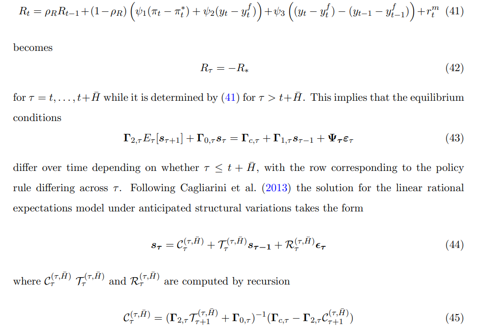
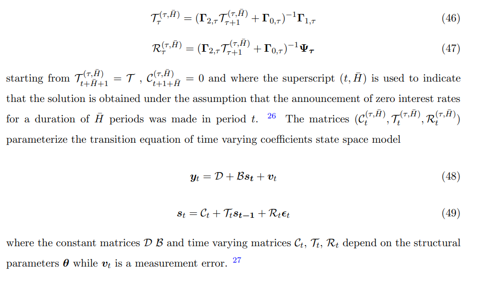
The New Keynesian model is the version of the Smets et al. (2007) model considered in Del Negro et al. (2015). The model features price and wage stickiness, investment adjustment costs, habit formation in consumption and 7 shocks being monetary policy shocks, technology shocks, price mark-up shocks, wage mark-up shocks, preference shocks, fiscal policy shock and shocks to the marginal efficiency of capital. In the model the monetary policy rule accounts for ZLB period and forward guidance.[25] More specifically, when accounting for the zero lower bound and forward guidance the solution of the model implies a state state space representation which exhibits time varying coefficients. The solution method follows the approach developed by Cagliarini et al. (2013) for linear stochastic rational expectations models in the face of a finite sequence of anticipated structural changes. In particular, it is assumed that at a given period t, agents expect the nominal interest rate to be at the ZLB for H¯ periods. That is, the monetary policy rule
4.2 Simulation study
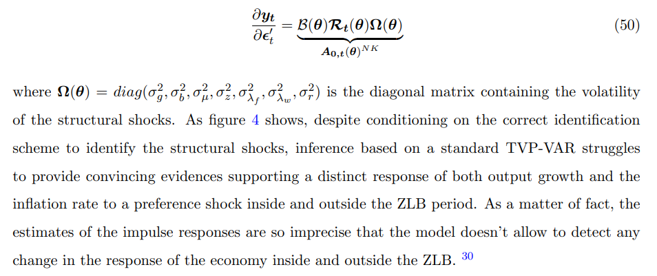
As anticipated above and shown in figure 3, the NK model predicts a distinct response of the economy to a demand shock inside and outside the ZLB period. Conditioning on the vector of deep parameters of the NK model, I simulate data from the state space representation (48) and (49). 28 In the simulation I consider artificial samples with T = 139 mimicking quarterly observations for the period 1985Q1-2019Q3. The length of the ZLB period is 28 quarters, covering the period 2009Q1-2015Q3. I estimate a standard TVP-VAR model (Chan et al. 2009) on the simulated data to understand whether the model is able to recover the change in the response of the economy during the ZLB period generated by the NK model.29 Figure 4 shows the estimated responses of output and inflation to a preference shock obtained from a standard TVP-VAR. The figure plots the responses of output growth (cumulative) and the inflation rate to a one standard deviation preference shock in two reference dates, one outside and the other one inside the ZLB period. In order to identify the shocks in the structural TVP-VAR I exploit the true impact matrix of the NK model given by
4.3 Estimating the TC-TVP-VAR on US data
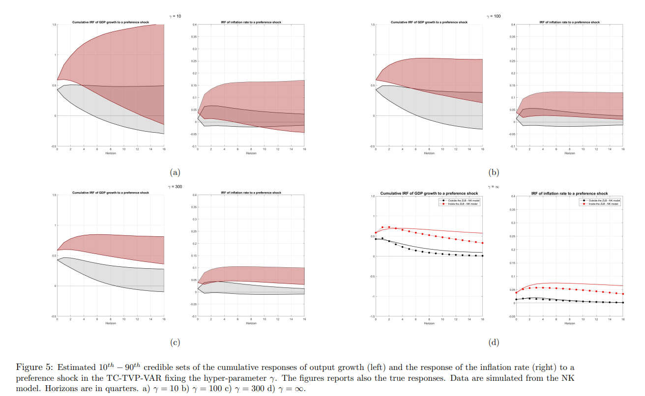
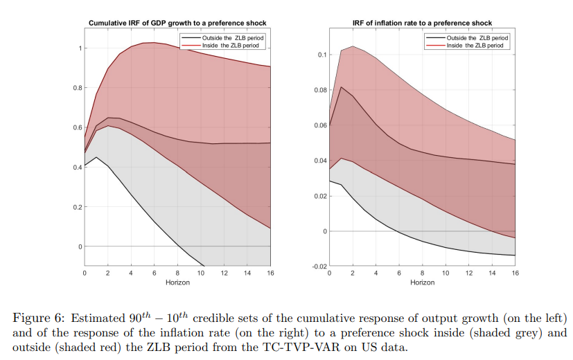
When analyzing real data, it is reasonable to think of the NK model just as an approximate (most likely misspecified) tightly parameterized representation of the true data generating process. In other words, we do not expect the restrictions implied by the NK model to hold exactly. However, when encoded into a prior, these restrictions might prove to be useful to get more precise estimates of the time varying coefficients and of nonlinear functions of these coefficients, such as the impulse response functions. In particular, in our context, shrinkage might turn out to be particularly useful to detect the change in the response of the economy during the ZLB period predicted by the NK model. In order to analyze to what extent the data support the changing behavior during the ZLB, my approach consists in exploiting the New Keynesian model as a prior for the TC-TVP-VAR. The extent to which the predictions from the New Keynesian model will be supported by the data will depend on the estimated posterior distribution of γ, the hyperparameter governing the degree of shrinkage of the parameters towards the restriction implied by the New Keynesian model. If the posterior distribution of γ is concentrated relatively far from zero, the coefficients of the TVP-VAR will be shrinked towards the restrictions implied by the NK model and the estimated responses from the TC-TVP-VAR will resemble the predictions of the NK model. This would happen in practice if the restrictions from the NK model find enough support on the data. Conversely, if the restrictions from the NK are deemed implausible by the data, the posterior distribution of γ will be concentrated around zero and the estimates of the time varying coefficients will not reflect the restrictions coming from the prior. The estimated model is a 7-variable TC-TVP-VAR for the US economy including output growth, consumption growth, investment growth, real wage growth, hours worked, inflation and the Fed Fund rate and it is estimated over the sample 1985Q1-2019Q3.32 In order to identify the shocks in the structural TVP-VAR, I exploit the impact matrix of the NK model. The deep parameters of the NK model are treated as unknown and estimated along with the other parameters of the model, which implies that on impact there is uncertainty on the effect of the shocks on the variables of the system. Figure 6 shows the estimated responses from the TC-TVP-VAR where the hyper-parameter γ is estimated along with the other parameters of the model. The posterior distribution of γ is estimated to be concentrated far from zero, meaning that the time varying restriction functions from the NK model find sufficient support on the data. This, in turns, is reflected on the estimates of the 10th−90th credible sets which provide some evidences supporting a distinct responses of the economy inside and outside the ZLB period. As predicted by the NK model, the estimates suggest that when monetary policy is constrained by the nominal rate hitting the ZLB, the preference shock is reabsorbed at a much slower pace by the economy. Following the positive demand shock both output growth and the inflation rate increase, with the effect on output growth being more precisely estimated at shorter horizons. The effect on output peaks after almost two quarters outside the ZLB period, while about after five quarters inside the ZLB period. As for inflation, the effect peaks after one quarter outside the ZLB period and after two quarters inside the ZLB period. After the peak, the effect of the preference shock on both output and inflation dies at a much slower pace inside the ZLB period, as foreseen by the NK model.
This paper is available on arxiv under CC 4.0 license.
[24.] In the model, the ZLB period is treated as in Del Negro et al. (2015), and more details on the model will be explained in the next subsection.
[25.] The log-linearized equilibrium conditions of the model can be found in the appendix A.3 The model is labelled ”SW” in Del Negro et al. (2015) and assumes a constant inflation target.
[26.] Following Del Negro et al. (2015) to measure the number of quarters H¯ that the Federal Funds Rate is expected to remain at the ZLB I exploit information based on the overnight index swap (OIS) rates. In particular I identify the ZLB period as the quarters in which the OIS rate is lower then 0.35. This classification leads to the same ZLB period considered in Benati et al. (2023) and Debortoli et al. (2019) namely 2009Q1-2015Q3 (28 quarters). Following Chen et al. (2012) I assume that the number of quarters such that the policy rate is expected to stay fixed, is at most equal to four.
[27.] Details for the observation equations are in the appendix A.3 together with the list of the deep structural parameters θ (appendix A.3.1).
[28.] Parameters are calibrated according to the posterior mode in Del Negro et al. (2015)
[29.] The standard TVP-VAR model is the model in Chan et al. (2009). To estimate the model I use the MATLAB codes kindly made available by Joshua Chan on his personal website.
[30.] As shown in the appendix in figure 8, this result is not driven by this specific simulated sample of artificial observations.
[31.] Also in this case, in the TC-TVP-VAR we condition on the correct identification scheme for the structural shocks.
[32.] Details on the variables and their transformation is available in the appendix A.3

