Author:
(1) David Staines.
Table of Links
4 Calvo Framework and 4.1 Household’s Problem
4.3 Household Equilibrium Conditions
4.5 Nominal Equilibrium Conditions
4.6 Real Equilibrium Conditions and 4.7 Shocks
5.2 Persistence and Policy Puzzles
6 Stochastic Equilibrium and 6.1 Ergodic Theory and Random Dynamical Systems
7 General Linearized Phillips Curve
8 Existence Results and 8.1 Main Results
9.2 Algebraic Aspects (I) Singularities and Covers
9.3 Algebraic Aspects (II) Homology
9.4 Algebraic Aspects (III) Schemes
9.5 Wider Economic Interpretations
10 Econometric and Theoretical Implications and 10.1 Identification and Trade-offs
10.4 Microeconomic Interpretation
Appendices
A Proof of Theorem 2 and A.1 Proof of Part (i)
B Proofs from Section 4 and B.1 Individual Product Demand (4.2)
B.2 Flexible Price Equilibrium and ZINSS (4.4)
B.4 Cost Minimization (4.6) and (10.4)
C Proofs from Section 5, and C.1 Puzzles, Policy and Persistence
D Stochastic Equilibrium and D.1 Non-Stochastic Equilibrium
D.2 Profits and Long-Run Growth
E Slopes and Eigenvalues and E.1 Slope Coefficients
E.4 Rouche’s Theorem Conditions
F Abstract Algebra and F.1 Homology Groups
F.4 Marginal Costs and Inflation
G Further Keynesian Models and G.1 Taylor Pricing
G.3 Unconventional Policy Settings
H Empirical Robustness and H.1 Parameter Selection
I Additional Evidence and I.1 Other Structural Parameters
I.3 Trend Inflation Volatility
C Proofs from Section 5
This section contains proof of the remaining propositions in Section 5, as well as additional supporting material and an extension of arguments concerning persistence.
C.1 Puzzles, Policy and Persistence
This subsection focuses on proving the main dynamics and policy results pertinent to first order dynamics.
C.1.1 Proof of Lemma A.1
Here is the proof of Chebyshev’s correlation inequality which is used to complete the proof of Proposition 5.

By assumptions placed on the measure, the first term can be decomposed into the (non-zero) contribution of terms above and below the expected value EV

(Strict) Monotonicity of U, V and the Lebesgue integral allow us to conclude that

Similarly when V is below average by the same argument

Now reversing yields

combining the numbered equations completes the proof.
C.1.2 Proof of Proposition 6
Proof. The planner can set interest rates to offset the demand shock ˆit = ψˆ t. This implements a non-stochastic steady state. Therefore the only remaining distortion is the markup of prices over marginal costs associated with imperfect competition. This can be remedied by a subsidy set to cancel the desired mark up as follows

with the optimal level

This creates an equivalence with the allocations of a standard competitive equilibrium. Therefore, these transfers can be funded by lump transfers thanks to Ricardian equivalence (see Barro [1974]).
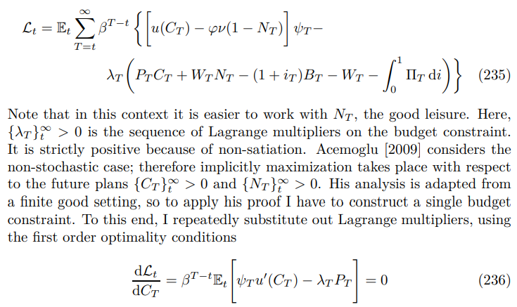
To apply this version of the welfare theorem, it is necessary to write the household’s problem as an infinite budget constraint, subject to the standard objective function (7). To do so consider the Lagrangian form of the problem from which the Euler is derived

In fact, the budget constraint can be given a particular compact form

where I have used the expression for the nominal discount factor

familiar from asset pricing literature. The final adjustment is to the measure of firms. He works with a finite number and therefore implicitly with the discrete measure, whereas here with a mean field of monopolistic competition in the background, we need to work with the standard Lebesgue measure.

Remark 37. Stokey [1989] provide an alternative treatment of welfare theorems, using production sets and allowing directly for stochasticity, from which an alternative proof might be developed.

Labor supply distortions have previously been a focus of business cycle accounting popular in the neoclassical tradition (see for example Chari et al. [2007] and Shimer [2009]). Although, inter-temporal labor substitution is somewhat controversial (see Bianchi et al. [2001] and Martínez et al. [2021]), it is likely some similar inter-temporal distortions would arise with any alternative microfoundations.
C.1.3 Proof of Proposition 8
Proof. This is a linear system of expectational equations, with two jump variables and no state variables. There are two cases to consider, one where there is a unique solution, the other where there is a multiplicity of solutions. When there is indeterminacy it will not be possible to rule out persistent fluctuations, arising from expectational bubbles. Later, when I connect the non-bifurcated approximation to the non-linear model, I will be able to rule out indeterminacy. The proof will be completed by showing that whenever there is a determinate solution it is non-persistent and that determinacy corresponds to the expression given in the proposition. To do so, I express the system in canonical form by substituting the Phillips curve and policy rule to form the canonical Euler. It can be expressed in the following matrix form

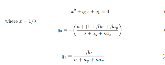
The condition for a unique solution is that we can solve the system forward. This requires both eigenvalues be outside the unit circle, as in Blanchard and Kahn [1980]. It is convenient to work with the inverse eigenvalue polynomial

LaSalle [2012] shows that there will be two inverse eigenvalues inside the unit circle if and only if

The second condition amounts to

which rearranges to give the desired expression. The second condition is redundant because

This paper is available on arxiv under CC 4.0 license.

