Author:
(1) David Staines.
Table of Links
4 Calvo Framework and 4.1 Household’s Problem
4.3 Household Equilibrium Conditions
4.5 Nominal Equilibrium Conditions
4.6 Real Equilibrium Conditions and 4.7 Shocks
5.2 Persistence and Policy Puzzles
6 Stochastic Equilibrium and 6.1 Ergodic Theory and Random Dynamical Systems
7 General Linearized Phillips Curve
8 Existence Results and 8.1 Main Results
9.2 Algebraic Aspects (I) Singularities and Covers
9.3 Algebraic Aspects (II) Homology
9.4 Algebraic Aspects (III) Schemes
9.5 Wider Economic Interpretations
10 Econometric and Theoretical Implications and 10.1 Identification and Trade-offs
10.4 Microeconomic Interpretation
Appendices
A Proof of Theorem 2 and A.1 Proof of Part (i)
B Proofs from Section 4 and B.1 Individual Product Demand (4.2)
B.2 Flexible Price Equilibrium and ZINSS (4.4)
B.4 Cost Minimization (4.6) and (10.4)
C Proofs from Section 5, and C.1 Puzzles, Policy and Persistence
D Stochastic Equilibrium and D.1 Non-Stochastic Equilibrium
D.2 Profits and Long-Run Growth
E Slopes and Eigenvalues and E.1 Slope Coefficients
E.4 Rouche’s Theorem Conditions
F Abstract Algebra and F.1 Homology Groups
F.4 Marginal Costs and Inflation
G Further Keynesian Models and G.1 Taylor Pricing
G.3 Unconventional Policy Settings
H Empirical Robustness and H.1 Parameter Selection
I Additional Evidence and I.1 Other Structural Parameters
I.3 Trend Inflation Volatility
E.3 Eigenvalue Conditions
This last part contains derivations of the two eigenvalue polynomials in the text, starting with the simplest limiting case and moving onto the general.
E.3.1 √ ε Characteristic Equation
Abstracting from the errors, the system can be written as follows

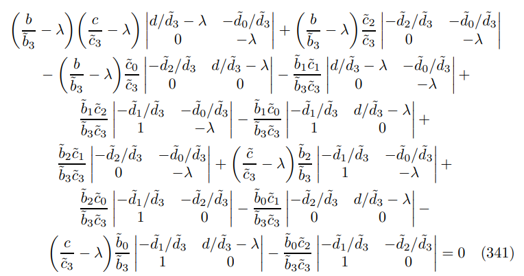
The characteristic polynomial comes from the following determinant equation

expressing in terms of minors gives

expanding out yields

then a simple rearrangement gives the expression in the text.
E.3.2 General Characteristic Equation
Start from the characteristic matrix

where I have reordered the variables (ˆπt, yˆt, ∆ˆ t, πˆt−1) ′ for convenience, substitution yields

expanding out the matrices gives

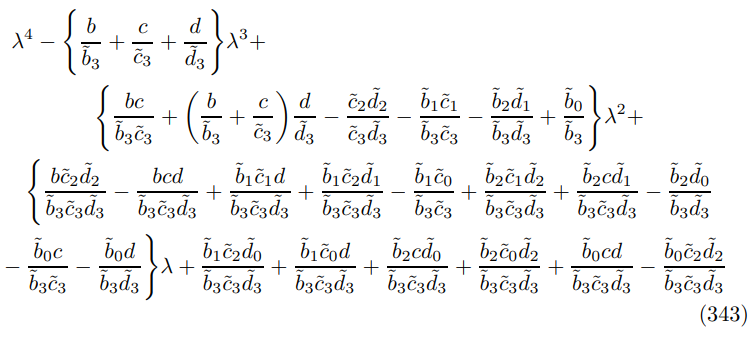
collecting terms implies the polynomial

where perhaps the most challenging step is the expansion

substituting in the ZINSS vanishing condition (138) yields the expression in Theorem 9.
This paper is available on arxiv under CC 4.0 license.

