Author:
(1) David Staines.
Table of Links
4 Calvo Framework and 4.1 Household’s Problem
4.3 Household Equilibrium Conditions
4.5 Nominal Equilibrium Conditions
4.6 Real Equilibrium Conditions and 4.7 Shocks
5.2 Persistence and Policy Puzzles
6 Stochastic Equilibrium and 6.1 Ergodic Theory and Random Dynamical Systems
7 General Linearized Phillips Curve
8 Existence Results and 8.1 Main Results
9.2 Algebraic Aspects (I) Singularities and Covers
9.3 Algebraic Aspects (II) Homology
9.4 Algebraic Aspects (III) Schemes
9.5 Wider Economic Interpretations
10 Econometric and Theoretical Implications and 10.1 Identification and Trade-offs
10.4 Microeconomic Interpretation
Appendices
A Proof of Theorem 2 and A.1 Proof of Part (i)
B Proofs from Section 4 and B.1 Individual Product Demand (4.2)
B.2 Flexible Price Equilibrium and ZINSS (4.4)
B.4 Cost Minimization (4.6) and (10.4)
C Proofs from Section 5, and C.1 Puzzles, Policy and Persistence
D Stochastic Equilibrium and D.1 Non-Stochastic Equilibrium
D.2 Profits and Long-Run Growth
E Slopes and Eigenvalues and E.1 Slope Coefficients
E.4 Rouche’s Theorem Conditions
F Abstract Algebra and F.1 Homology Groups
F.4 Marginal Costs and Inflation
G Further Keynesian Models and G.1 Taylor Pricing
G.3 Unconventional Policy Settings
H Empirical Robustness and H.1 Parameter Selection
I Additional Evidence and I.1 Other Structural Parameters
I.3 Trend Inflation Volatility
9.5 Wider Economic Interpretations
The final component of the section provides wider application and economic context to the mathematical objects and arguments developed here.
1. Invertibility The idea of the Grobman-Hartman theorem for trajectories and inverse function theorems[85] for mappings is that linear approximations can be used to represent local behavior because the system is invertible. Invertibility breaks down at ZINSS because the singular surfaces restrict the value of past variables, that otherwise determine the qualitative behavior of the cocycle, in the vicinity of ZINSS. This is most clear for (3) and (4) but as will become clear in the next section, it is also the case for (5).
2. Covers and Polydromy Whether price dispersion is first or second order around ZINSS depends on which limiting metric is used. This is a new idea to economists. The reason is that unlike the other two in Theorem 6, this cover is unramified by any singularity because around ZINSS it can be written in static form, going back to Proposition 3. The |ε| limit can be viewed as the volatile regime, whilst √ ε is the stable regime where the effect of inflation volatility has vanished. It should prove useful to study the dynamic role of price dispersion absent its static effects. Results are likely to extend to wide class of models with real rigidity.
Furthermore, |ε| limit is a natural way to incorporate volatility in trend inflation. The empirical evidence, considered in Appendix I.3, appears mixed on whether trend inflation shocks have first order dynamic effects. Therefore, I advise subsequent papers consider both until decisive evidence appears.
Moreover, the result has immediate econometric and computational implications. Informally, the |ε| small noise limit encompasses its counterpart √ ε, the very small noise limit. This makes it the more precise approximation in computational terms and the robust model in an econometric sense.
Alternatively, it introduces the possibility, albeit limited, for multiple equilibria back into DSGE. In fact, in Section 11, I show that this will always be the case because the equilibrium existence conditions will be the same for both. This result is general because price dispersion behaves as an error term around ZINSS.
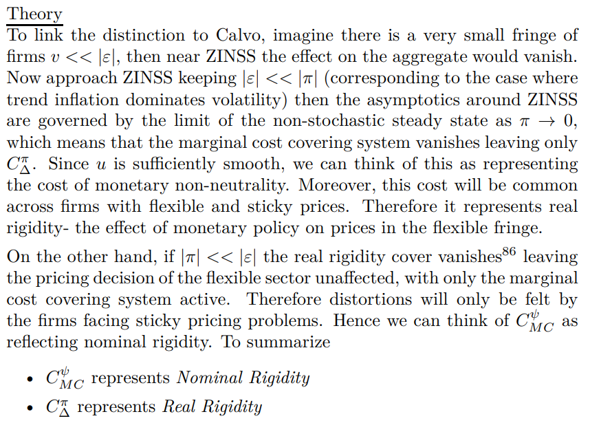
3. Covers and Rigidity Two of the covers from Theorem 6 have special significance to a longstanding macroeconomic debate. Ball and Romer [1990] decomposes the effect of monetary policy in a Keynesian model into two forces; nominal rigidity and real rigidity. Real rigidity is the effect of monetary non-neutrality on the behavior of flexible price firms, whilst nominal rigidity only pertains to those who have sticky prices. This dichotomy yields both theoretical and empirical implications.

The results speak to an old debate about the interplay between Classical and Keynesian distortions. The weak relationship between price dispersion and inflation and the promising hybrid structure of the √ ε Phillips curve belie the claim in Ball and Romer [1990] that real rigidity is required to fit the business cycle evidence and make the effects of monetary policy substantive. This underlines the importance of time as opposed to mere state dependence when modelling monetary policy, which was the basis for his claims.[87] A more complete analysis will appear in the empirical companion paper to follow.
4. Covers and Market Failures Moreover, the covering systems can be seen through a welfare economics lens, more akin to microeconomics. The nominal rigidity system could reflect individual failure on the part of the firms with rigid prices, in the terminology of Barile et al. [2017] (see also Bernheim [2009] and Bernheim [2016]). Otherwise, it could be institutional or governance failures; note perspectives from Vives [ed.] and Tirole [2010].[88] On the other hand, real rigidity here reflects coordination failure, a traditional theme in macroeconomics (see Cooper and John [1988] and Leijonhufvud [1968]).
5. Homology and Missing Equilibrium This explains how the limiting equilibrium Phillips curve (π, |ε|) → 0 represents a limiting equilibrium that is "missing" from the tangent space, like a vein in a rock.
6. Discretization Small noise limiting equilibrium constructions are robust to discretization, in a certain sense. Suppose the continuous stochastic processes in Section 4.8 and employed throughout the paper were replaced by a non-degenerate discrete process. Now suppose the maximum distance between any two realizations of the shocks were ε. The limit |ε| → 0 would recover our limiting equilibrium. Therefore, the results here can be seen as approximating regime switching frameworks, such as Hamilton [1989] and Hamilton [2010], which might be surprising.
7. Lucas Critique Figure 1 represents "passing the Lucas critique" with respect to the microfoundations criterion.
8. Double Bifurcation Around ZINSS there is a double bifurcation in the local ring system, associated with gluing together all the linear approximations to stochastic and non-stochastic equilibria. There is a trend inflation bifurcation

that economists have been aware of since Ascari and Rankin [2002]. However, there is an additional stochastic bifurcation as the size of the error term drops to zero.

It is this bifurcation that economists have been unaware of, which is causing all the approximations from the existing framework to give erroneous results. Some confusion may arise because a second order difference between lag polynomial roots is causing a first order bifurcation. This is certainly an unusual geometrical pathology.

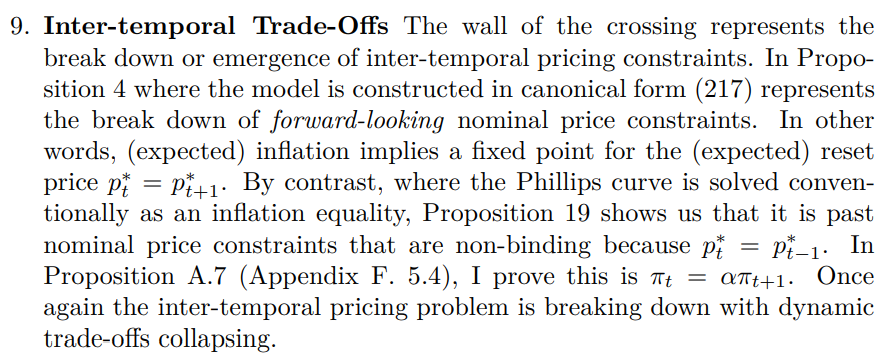
10. Codimensionality The ambient space has codimension one, in the sense that if you adjust one variable you move inside the singular surface (around ZINSS (3) implies this will be either current inflation or its lag). This ensures that the breakdown of inter-temporal pricing constraints "causes" the bifurcation. This would not increase however many other variables I added to flesh out the description of the supply side.
Arguably, the main interest for established economists is the codimension of the singular surface. This represents how many coefficients change when you move from the existing singular approximation (1) to the "correct" approximation (2). It is easy to see that this is equal to the dimension of the full space. One can think of the codimension of the singular surface less the codimension of the nonsingular surface as measuring the "size" of the bifurcation. It is a measure of how unrepresentative the ZINSS approximation is.
For our model this size is maximal. In some sense this is the worst possible pathology. It is impossible to learn anything from the existing approximation because there is no component of the Phillips curve unaffected. Staggered optimization creates a whole new transmission mechanism for monetary policy analysis. This will enable me to overturn the existence and stabilization properties of the model in Section 11, compared to Rotemberg back in Theorem 5. We can view the second dimension of the hole as representing the inter-temporal trade-offs, associated with the Euler equation and the cost channel, inherently, arising from the presence of lag terms. It links the "hole within a hole" back to the error symmetry, appearing at a steady state free from inter-temporal distortions.
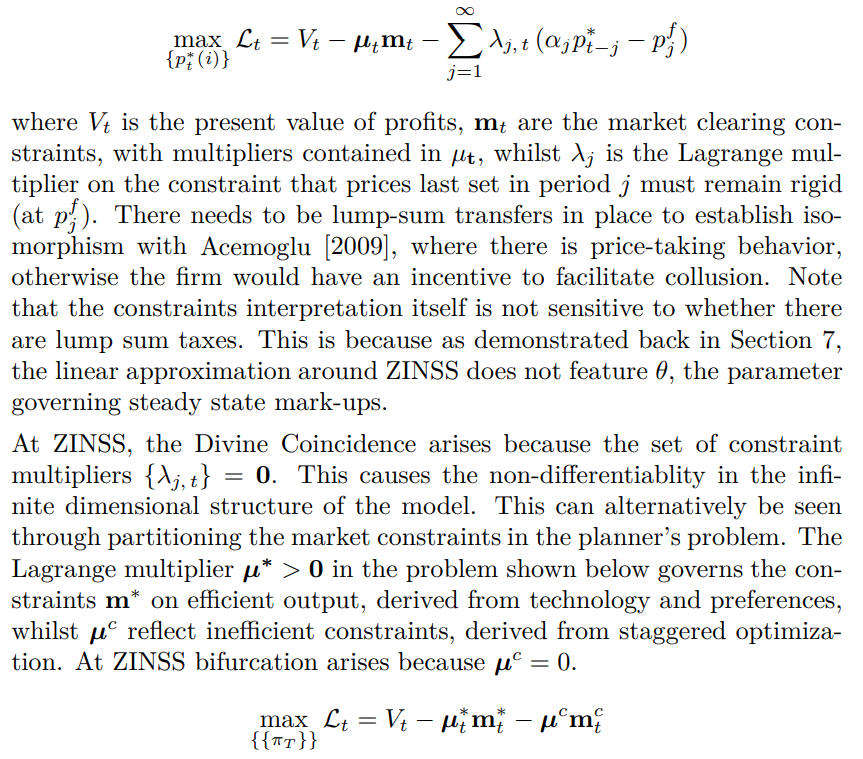
11. Constraints and Efficiency The system of singularities are constraints imposed on the social planner or equivalently the representative firm of Acemoglu [2009] by the economy’s history of non-optimizing behavior.
Formally, the representative firms problem takes the form

The break down of all these constraints simultaneously is the "Coincidence" behind the "Divine Coincidence". This completes the optimization theoretic account of the standard Calvo model around ZINSS.
Divine Coincidence is intimately tied up with the infinite horizon of the Calvo optimization problem. With heterogeniety in the pricing process of firms, it can be seen as of infinite codimension because just one measure of constrained firms would create market failure. This has practical implications, for example where price spells are truncated, as is common in empirical work.[89] Around ZINSS there would always be a positive constraint multiplier on the firms forced to reset their prices so there would be no Divine Coincidence. In general, heterogeneity can increase the size of the bifurcation by raising codimension of the singular surface, without changing the dimension of the wall.[90]
12. Mathematical Economics The results in this paper have demonstrated that the distinction between mathematics and physics, where physicists theorize and make conjectures, whilst mathematicians provide rigorous proofs, will not work for economics. DSGE and most other economic models are over-identified (possess negative degrees of freedom). This means that loose conjectures are liable to prove untrue and economists need to be aware of analytical pathologies. This should provide fertile ground for future collaboration between economists and mathematicians.
This paper is available on arxiv under CC 4.0 license.
[85] Unlike Grobman-Hartman there are inverse function theorems for discontinuous derivatives but they presuppose the derivative is locally invertible, which is missing here (see https://terrytao.wordpress.com/2011/09/12/the-inverse-function-theorem-foreverywhere-differentiable-maps/).
[86] This argument is a little more difficult to motivate; it would arise if the volatility of output were to dominate the volatility of inflation. Heuristically, imagine a static aggregate demand and supply model. This would correspond to instances where the supply curve is considerably steeper than the aggregate demand schedule. Alternatively, one could strike out price dispersion a priori with the motivation discussed earlier.
[87 An alternative less formal take on real rigidity has it flattening the Phillips curve. This will come up in the next section. The conclusions will not change.
[88] Alternatively, it could be viewed as pro-social behavior on the part of the firm, as in Rotemberg [2011]. This is arguably a more significant avenue for future applied research.
[89] Consider, for example, the Generalized Taylor formulation of Dixon [2012] and Dixon and Le Bihan [2012], which approximates heterogeneous price adjustment with contracts of finite length that differ between firms. They show that these can arbitrarily well approximate the reset distribution under the standard Calvo here.
[90] In fact, the bifurcation would theoretically be infinite dimensional if we used a nonparametric function to estimate the reset price probability.

