Author:
(1) David Staines.
Table of Links
4 Calvo Framework and 4.1 Household’s Problem
4.3 Household Equilibrium Conditions
4.5 Nominal Equilibrium Conditions
4.6 Real Equilibrium Conditions and 4.7 Shocks
5.2 Persistence and Policy Puzzles
6 Stochastic Equilibrium and 6.1 Ergodic Theory and Random Dynamical Systems
7 General Linearized Phillips Curve
8 Existence Results and 8.1 Main Results
9.2 Algebraic Aspects (I) Singularities and Covers
9.3 Algebraic Aspects (II) Homology
9.4 Algebraic Aspects (III) Schemes
9.5 Wider Economic Interpretations
10 Econometric and Theoretical Implications and 10.1 Identification and Trade-offs
10.4 Microeconomic Interpretation
Appendices
A Proof of Theorem 2 and A.1 Proof of Part (i)
B Proofs from Section 4 and B.1 Individual Product Demand (4.2)
B.2 Flexible Price Equilibrium and ZINSS (4.4)
B.4 Cost Minimization (4.6) and (10.4)
C Proofs from Section 5, and C.1 Puzzles, Policy and Persistence
D Stochastic Equilibrium and D.1 Non-Stochastic Equilibrium
D.2 Profits and Long-Run Growth
E Slopes and Eigenvalues and E.1 Slope Coefficients
E.4 Rouche’s Theorem Conditions
F Abstract Algebra and F.1 Homology Groups
F.4 Marginal Costs and Inflation
G Further Keynesian Models and G.1 Taylor Pricing
G.3 Unconventional Policy Settings
H Empirical Robustness and H.1 Parameter Selection
I Additional Evidence and I.1 Other Structural Parameters
I.3 Trend Inflation Volatility
11 Policy Rule
Here I prove the anti-Taylor policy rule and briefly outline its significance.
Theorem 9. There exists polydromy if and only if aπ < 1, otherwise there is no solution at all.

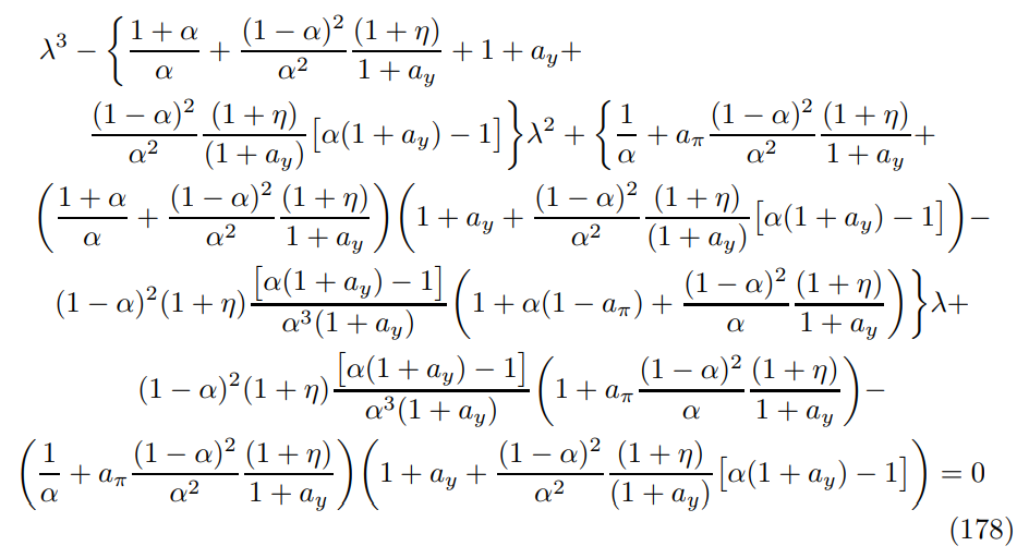
this expands out to

which simplifies to

It is clear that λ = 1/α is a root- which will lie outside the unit circle. The equation factorizes to

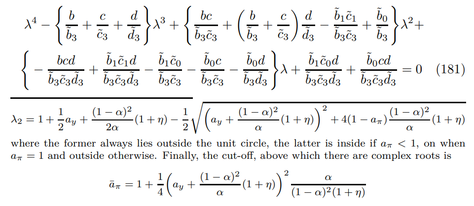
Together Theorem 3 and Proposition 16 stipulate that a solution exists if and only if the quadratic contains precisely one root inside the unit circle. This rules out complex roots. The sign pattern rules out negative roots. Therefore, the cut-off must be associated with λ = 1 which is clearly associated with aπ = 1. Rouche’s theorem implies that when aπ is sufficiently large there will be no roots inside the unit circle. Hence the desired configuration must be associated with aπ < 1.[102]
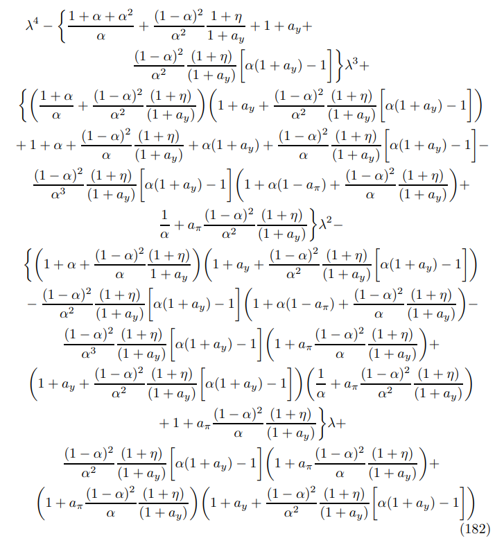
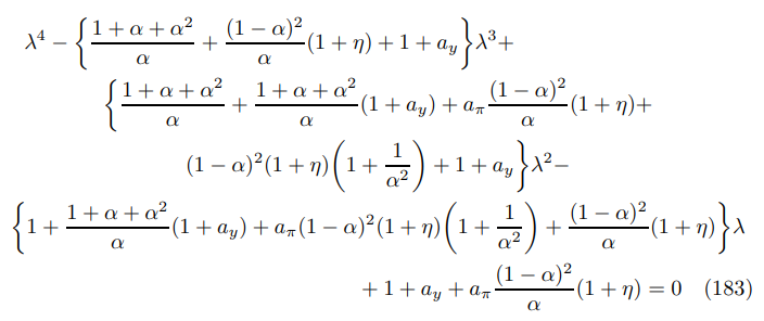
The extension to |ε| is straightforward. Its eigenvalue equation is


This simplifies to

Plugging in reveals that there is one root inside the unit circle at λ = α and another outside at λ = 1/α. When the polynomial is factorized, the other roots come from the same quadratic equation as in the √ ε limit in (180). There have to be two roots inside the unit circle overall, so the parameter condition is identical.
There might be a wider lesson for general equilibrium theory and mathematical economics. Equilibrium existence is demanding a contraction on destabilizing general equilibrium effects. To see how, consider the following decomposition of the lagged inflation coefficient informed by Decomposition 1.
Decomposition 2.

where GE represents the general equilibrium impulse from the cost channel

whilst the unitary terms come from the wall of the crossing (A) and the α comes from the singular component (D) and (F) from Decomposition 1.

Turning to the New Keynesian field in particular, the following observation should prove interesting for empirical specification design, as well as theoretical consideration of the property of structural disturbances.
Remark 35. Note that down the |ε| limit ∆ detaches from the rest of the system and behaves as an exogenous variable, like the cost-push shocks previously used to drive the Phillips curve.
I anticipate the policy rule results will generalize widely and may extend out to moderate rates of trend inflation. To reaffirm, in economic terms the blow up is unproblematic and even instructive. On the one hand, the economy is stable under inactive settings, when the Taylor rule represents a realistic shorthand description of monetary policy-making. On the other hand, the model explodes under active policy, precisely when following a simple rule is most unrealistic. Successful central banks employ macroeconomists and other skilled practitioners in order to implement a semblance of optimal monetary policy. Best practice appears to be inertial. In time, I expect the theory of monetary policy to catchup.[103]
Finally, there is a direct connection between ex post constraints implied by the existence conditions and ex ante constraints breaking Divine Coincidence. The policies that are ruled out ex post, which seek to raise real interest rates immediately, are precisely those that fail to engage with the ex ante restrictions that give the economy inertia. Elaborate mathematical machinery serves to rule out evidently unsustainable macroeconomic policies. I anticipate this will become a universal lesson in New Keynesian economics.
This paper is available on arxiv under CC 4.0 license.


