Author:
(1) David Staines.
Table of Links
4 Calvo Framework and 4.1 Household’s Problem
4.3 Household Equilibrium Conditions
4.5 Nominal Equilibrium Conditions
4.6 Real Equilibrium Conditions and 4.7 Shocks
5.2 Persistence and Policy Puzzles
6 Stochastic Equilibrium and 6.1 Ergodic Theory and Random Dynamical Systems
7 General Linearized Phillips Curve
8 Existence Results and 8.1 Main Results
9.2 Algebraic Aspects (I) Singularities and Covers
9.3 Algebraic Aspects (II) Homology
9.4 Algebraic Aspects (III) Schemes
9.5 Wider Economic Interpretations
10 Econometric and Theoretical Implications and 10.1 Identification and Trade-offs
10.4 Microeconomic Interpretation
Appendices
A Proof of Theorem 2 and A.1 Proof of Part (i)
B Proofs from Section 4 and B.1 Individual Product Demand (4.2)
B.2 Flexible Price Equilibrium and ZINSS (4.4)
B.4 Cost Minimization (4.6) and (10.4)
C Proofs from Section 5, and C.1 Puzzles, Policy and Persistence
D Stochastic Equilibrium and D.1 Non-Stochastic Equilibrium
D.2 Profits and Long-Run Growth
E Slopes and Eigenvalues and E.1 Slope Coefficients
E.4 Rouche’s Theorem Conditions
F Abstract Algebra and F.1 Homology Groups
F.4 Marginal Costs and Inflation
G Further Keynesian Models and G.1 Taylor Pricing
G.3 Unconventional Policy Settings
H Empirical Robustness and H.1 Parameter Selection
I Additional Evidence and I.1 Other Structural Parameters
I.3 Trend Inflation Volatility
A.3 Proof Part (iii)
This part proves the claim concerning output.

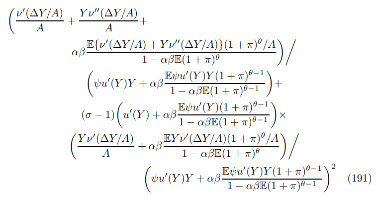
Note that the condition is sharp in θ, by considering the limits respectively as α → 0 and π → −100%. Now the Jensen-Chebyshev inequality implies that the left-hand side strictly exceeds the right-hand side, evaluated at the non-stochastic steady state. This implies that ∆ or Y must differ from their non-stochastic steady state values to restore equilibrium. The right-hand side is clearly increasing in ∆. Therefore to correct the imbalance ∆ would have to fall. However, this induces a contradiction since ∆ is convex in π for the relevant parametization. Hence Y must change to equilibriate the system. To see that it must fall take the derivative of the right-hand side

since when σ ≥ 1 the second term is non-negative and therefore unable to cancel the strictly positive first term.
Sharpness depends on parametric assumptions. Suppose 0 < σ < 1 and consider the joint limit, where the economy approaches any non-stochastic steady state and A → 0. There are two competing terms. The first represented by the top two lines above is always positive and the second is negative by assumption.
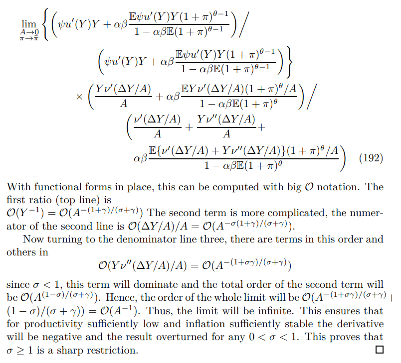
The idea is to show that sufficiently close to these limiting cases the second term will dominate. To achieve this consider the ratio of the negative term to the positive term. The proof will be complete if its limit is greater than unity.
The expression is the following product

This paper is available on arxiv under CC 4.0 license.

