Author:
(1) David Staines.
Table of Links
4 Calvo Framework and 4.1 Household’s Problem
4.3 Household Equilibrium Conditions
4.5 Nominal Equilibrium Conditions
4.6 Real Equilibrium Conditions and 4.7 Shocks
5.2 Persistence and Policy Puzzles
6 Stochastic Equilibrium and 6.1 Ergodic Theory and Random Dynamical Systems
7 General Linearized Phillips Curve
8 Existence Results and 8.1 Main Results
9.2 Algebraic Aspects (I) Singularities and Covers
9.3 Algebraic Aspects (II) Homology
9.4 Algebraic Aspects (III) Schemes
9.5 Wider Economic Interpretations
10 Econometric and Theoretical Implications and 10.1 Identification and Trade-offs
10.4 Microeconomic Interpretation
Appendices
A Proof of Theorem 2 and A.1 Proof of Part (i)
B Proofs from Section 4 and B.1 Individual Product Demand (4.2)
B.2 Flexible Price Equilibrium and ZINSS (4.4)
B.4 Cost Minimization (4.6) and (10.4)
C Proofs from Section 5, and C.1 Puzzles, Policy and Persistence
D Stochastic Equilibrium and D.1 Non-Stochastic Equilibrium
D.2 Profits and Long-Run Growth
E Slopes and Eigenvalues and E.1 Slope Coefficients
E.4 Rouche’s Theorem Conditions
F Abstract Algebra and F.1 Homology Groups
F.4 Marginal Costs and Inflation
G Further Keynesian Models and G.1 Taylor Pricing
G.3 Unconventional Policy Settings
H Empirical Robustness and H.1 Parameter Selection
I Additional Evidence and I.1 Other Structural Parameters
I.3 Trend Inflation Volatility
5.3 Two Comparison Models
This subsection introduces two alternative models featuring monetary Non neutrality. They will be used in the next section and throughout the paper as a point of comparison with solutions of the Calvo model. The first model is classical, in the sense that it features perfectly flexible prices. The second is Keynesian because prices are not able to adjust fully to inflation. Along with the menu cost model discussed in Section 8, it is an example of a state-dependent pricing model. Crucially, it does not feature staggered optimization. Prices will typically change in every period. I layout the equivalence between the existing solution of Calvo and the Rotemberg model, I extend this equivalence to the original Lucas model, allowing me to view it as part of the observational equivalence claim of Lucas Jr [1976]. Finally, I briefly review the rest of the critique.
5.3.1 Lucas Model
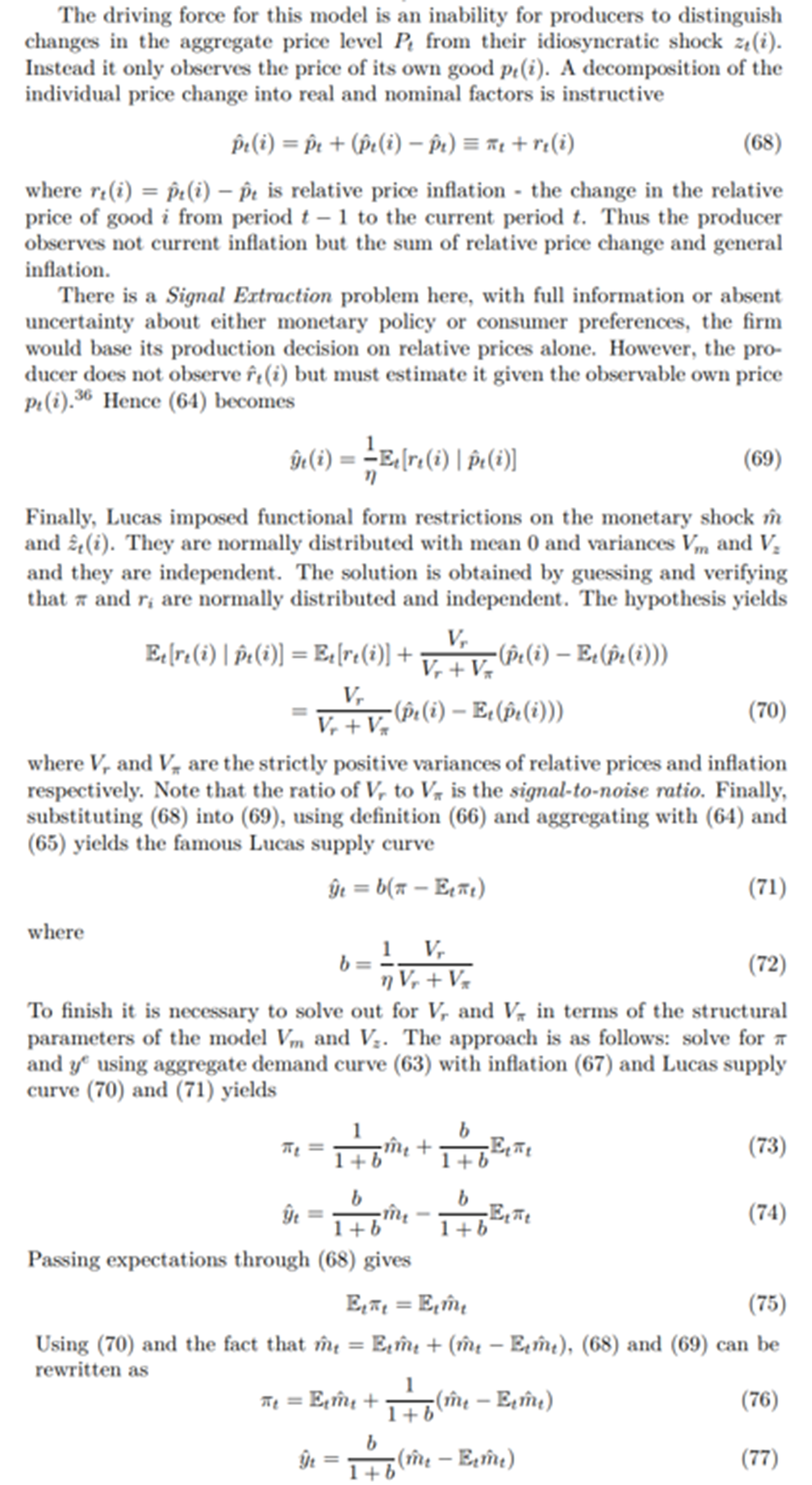
Lucas Jr [1972] is the original rational expectations monetary model. Markets are perfectly competitive and anticipated monetary shocks are impotent. Monetary non-neutrality arises because of imperfect information rather than sticky prices. Nevertheless, by adding a money demand function, I am able to derive surprising similarity to New Keynesian models with price rigidity.
There are a collection of price-taking households.[34] Each produces a single good, using just its own labor.[35] The choice problem simplifies to a static labor-leisure trade-of

The first order condition balances marginal revenue and marginal cost so

Solving and log-linearizing gives an expression for an individual firm’s supply curve

For parsimony, a reduced form aggregate demand curve replaces the Euler equation (18).

Idiosyncratic taste shocks, reflected by the disturbance zt(i) in the individual firms demand schedule, are essential to the Lucas model. I assume they are independent and identically distributed across producers and time, with tail restrictions such that they will cancel out in aggregate almost surely. Here is the log-linear form

There is linear aggregation so

whilst

Monetary non-neutrality is entirely driven by unexpected shocks. There is no role for price dispersion here, since the firms are price-takers and the distribution of relative price is unaffected by inflation. Unlike its Keynesian counterparts, the Lucas model would be unaffected by trend inflation.

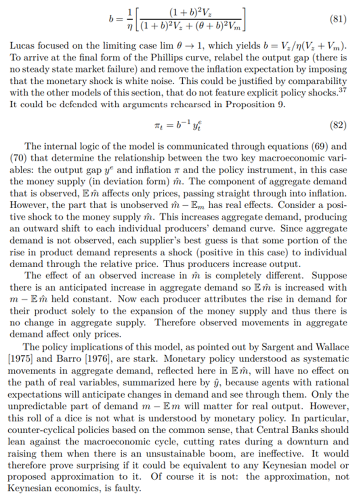
Using the individual supply curve (62), demand curve (64), steady state deviation (68) and the Lucas supply curve, (71) and (72) implies the expression for relative price deviation

and from (69) and (70)

This allows me to derive the following implicit formulation final form for the slope of the Lucas surprise Phillips curve

5.3.2 Rotemberg Pricing
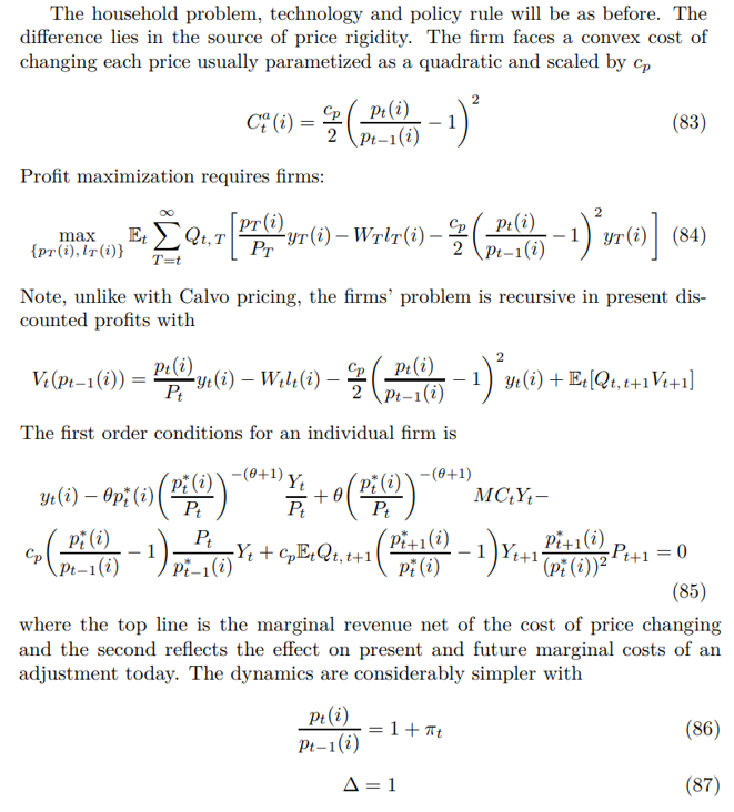
This model Rotemberg [1982] is perhaps the simplest formulation of state dependent pricing and the one most commonly compared to Calvo. The idea is that firms face a convex cost of changing prices and therefore they do not adjust immediately to their optimal flexible price. The problem is that convex costs of price changing imply firms change their prices every period through small adjustments. This runs contrary to an overwhelming body of evidence of infrequent large adjustment discussed in Appendix H.1.3.

Therefore the first order conditions simplify to

Finally, the resource constraint reflecting a wedge between production and consumption caused by the cost of price changing replaces (20)

Author:
(1) David Staines.
This paper is available on arxiv under CC 4.0 license.
[34] It is not common to have differentiated products and price-taking behavior. For motivation imagine there were actually multiple households producing the same good and therefore competition between them or the possibility to set-up firms with a consequent free entry condition. Recall the Bertrand paradox that two competing firms can implement a competitive equilibrium.
[35] This formulation comes from Romer [2012]. The idea is to avoid the households using the economy-wide labor market to deduce the aggregate price level. In the original paper, Lucas used an overlapping generations structure where households produced in one period then sold output in the next. Recent literature has developed more sophisticated stories about dispersed private information and strategic interaction. I do not pursue this approach as I am looking for a benchmark model.

