Table of Links
4 Calvo Framework and 4.1 Household’s Problem
4.3 Household Equilibrium Conditions
4.5 Nominal Equilibrium Conditions
4.6 Real Equilibrium Conditions and 4.7 Shocks
5.2 Persistence and Policy Puzzles
6 Stochastic Equilibrium and 6.1 Ergodic Theory and Random Dynamical Systems
7 General Linearized Phillips Curve
8 Existence Results and 8.1 Main Results
9.2 Algebraic Aspects (I) Singularities and Covers
9.3 Algebraic Aspects (II) Homology
9.4 Algebraic Aspects (III) Schemes
9.5 Wider Economic Interpretations
10 Econometric and Theoretical Implications and 10.1 Identification and Trade-offs
10.4 Microeconomic Interpretation
Appendices
A Proof of Theorem 2 and A.1 Proof of Part (i)
B Proofs from Section 4 and B.1 Individual Product Demand (4.2)
B.2 Flexible Price Equilibrium and ZINSS (4.4)
B.4 Cost Minimization (4.6) and (10.4)
C Proofs from Section 5, and C.1 Puzzles, Policy and Persistence
D Stochastic Equilibrium and D.1 Non-Stochastic Equilibrium
D.2 Profits and Long-Run Growth
E Slopes and Eigenvalues and E.1 Slope Coefficients
E.4 Rouche’s Theorem Conditions
F Abstract Algebra and F.1 Homology Groups
F.4 Marginal Costs and Inflation
G Further Keynesian Models and G.1 Taylor Pricing
G.3 Unconventional Policy Settings
H Empirical Robustness and H.1 Parameter Selection
I Additional Evidence and I.1 Other Structural Parameters
I.3 Trend Inflation Volatility
6 Stochastic Equilibrium
This section defines and develops the stochastic equilibrium methodology that forms the backbone of this paper. There are four subsections. The first provides a short background in the underlying mathematical disciplines of ergodic theory and random dynamical systems, with immediate application to our context. The second explicitly constructs the equilibrium. The third compares it with existing informal concepts in the literature. The fourth shows how stochastic equilibrium surfaces can be used to derive global properties of economic and mathematical importance.
6.1 Ergodic Theory and Random Dynamical Systems
I will use ergodic theory, the branch of mathematics that studies the long run behavior of dynamical systems to build the novel equilibrium concept. It is necessary to present several definitions integral to ergodic theory and dynamical systems, as well as clarifying aspects of the mathematical environment.
6.1.1 Random Dynamical Systems
This part is prerequisite for understanding ergodic theory. It sheds light on some of the errors discussed in the previous section, which revealed popular confusion about the properties of the underlying probabilistic system.
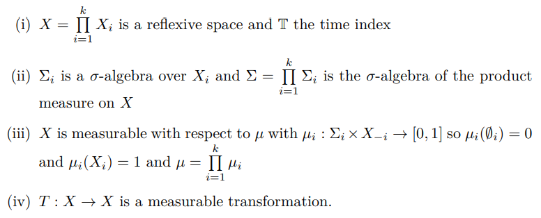
Definition 1. A measure-preserving dynamical system is defined as a probability space with a measure-preserving transform.
(X, T, Σ, µ, T)
such that

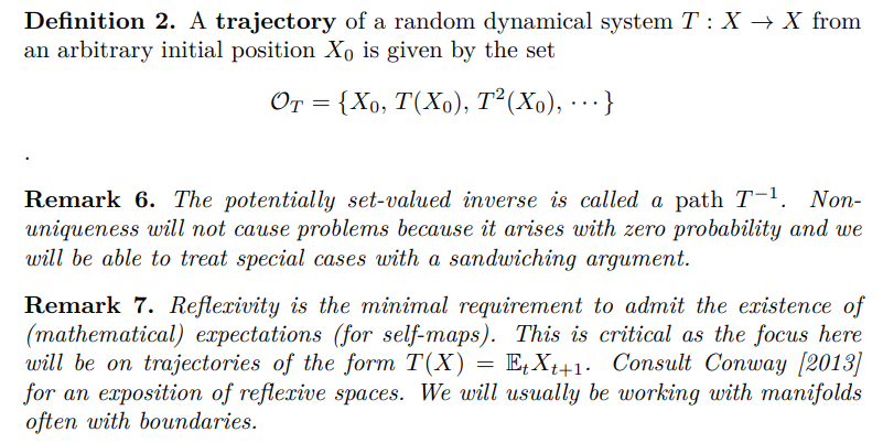
To analyze the time evolution of the system I introduce

6.1.2 Ergodicity
The following attributes characterize ergodicity:
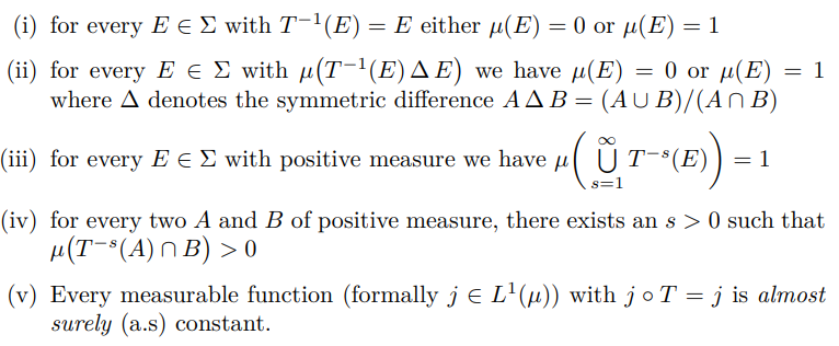
Definition 3. Let (X, Σ, µ) and T : X → X be a measure-preserving transformation. We say that T is ergodic with respect to µ (or alternatively that µ is ergodic with respect to T) if one of the following equivalent statements is true

Intuitively, ergodicity is the property that a system forgets its initial position and that it has well-defined long-run behavior. It is a property of the system as a whole or a subset that behaves as a component of the whole process. Conditions (ii)-(iv) state that if you move far enough back or forward in time (almost) any two positions of the system will occur in probability. Aliprantis and Border [2007] Theorem 20.7 provides a proof that these conditions are equivalent.
For Markov chains, ergodic measures have a powerful uniqueness property. Although, a state space may have multiple ergodic sets, a given ergodic set can only possess one ergodic measure, for proof consult Hairer [2018] Theorem 5.7 p. 40-42. Part (iv) can be interpreted as a weak restriction on hysteresis, that is intuitive in a business cycle context. The final part is the long run equilibrium property. It implies that the ergodic measure sets all moments to their long term values. The "almost sure" aspect allows us to associate it with a point in space as we would a non-stochastic steady state.

To analyze dynamics and stability properties of equilibrium it is necessary to introduce stronger restrictions known as mixing condition:
Definition 5. For a measure-preserving transform T : X → X the following are defining conditions for every A, B ∈ Σ
i Strong Mixing

ii Weak Mixing

iii Ergodic

Proposition 12. (Ergodic Hierarchy)
Strong Mixing ⇒ Weak Mixing ⇒ Ergodicity
Proof. Provided by Theorem 20.11 and Corollary 20.12 (p 662-664) in Aliprantis and Border [2007].

The final result clarifies that an ergodic measure sends all (non-divergent) moments to their long run equilibrium values. It should be of general economic interest and application.

Consult Hairer [2018] Theorem 5.2 p 38-40 for a proof.
Author:
(1) David Staines.
This paper is available on arxiv under CC 4.0 license.


