Table of Links
4 Calvo Framework and 4.1 Household’s Problem
4.3 Household Equilibrium Conditions
4.5 Nominal Equilibrium Conditions
4.6 Real Equilibrium Conditions and 4.7 Shocks
5.2 Persistence and Policy Puzzles
6 Stochastic Equilibrium and 6.1 Ergodic Theory and Random Dynamical Systems
7 General Linearized Phillips Curve
8 Existence Results and 8.1 Main Results
9.2 Algebraic Aspects (I) Singularities and Covers
9.3 Algebraic Aspects (II) Homology
9.4 Algebraic Aspects (III) Schemes
9.5 Wider Economic Interpretations
10 Econometric and Theoretical Implications and 10.1 Identification and Trade-offs
10.4 Microeconomic Interpretation
Appendices
A Proof of Theorem 2 and A.1 Proof of Part (i)
B Proofs from Section 4 and B.1 Individual Product Demand (4.2)
B.2 Flexible Price Equilibrium and ZINSS (4.4)
B.4 Cost Minimization (4.6) and (10.4)
C Proofs from Section 5, and C.1 Puzzles, Policy and Persistence
D Stochastic Equilibrium and D.1 Non-Stochastic Equilibrium
D.2 Profits and Long-Run Growth
E Slopes and Eigenvalues and E.1 Slope Coefficients
E.4 Rouche’s Theorem Conditions
F Abstract Algebra and F.1 Homology Groups
F.4 Marginal Costs and Inflation
G Further Keynesian Models and G.1 Taylor Pricing
G.3 Unconventional Policy Settings
H Empirical Robustness and H.1 Parameter Selection
I Additional Evidence and I.1 Other Structural Parameters
I.3 Trend Inflation Volatility
6.2 Equilibrium Construction
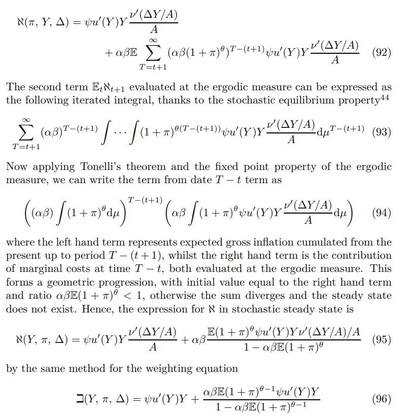
Here I characterize the stochastic equilibrium of the Calvo New Keynesian economy. The main tool is Birkhoff’s ergodic theorem. The stochastic steady state resembles its non-stochastic counterpart, except there are expectation terms attached to future realizations of non-linear functions of the variables (π, y, ∆, ψ, A) underpinning the recursive equilibrium, described back in Section 4.8 and Proposition 4. Current values of this set can be interpreted as their long run mathematical expectation. Existence results will be established in Section 8.
Starting with the Phillips curve, in particular the numerator of the reset price relationship from Proposition 1 given by combining infinite horizon expression (28) and recursive form (30)

combining gives the basis for the Stochastic Equilibrium Phillips curve.

Price dispersion evolves as follows

It is clear that the asymptote in all these equations corresponds to the case where ∆ grows unbounded. The Euler equation takes the form

Hence the equilibrium real interest rate, known as the natural rate of interest rate, is

Similar expressions could be written for the quantities U and Π but are suppressed in the interest of space.
Author:
(1) David Staines.
This paper is available on arxiv under CC 4.0 license.
[44] This integral is technically a Bochner or strong integral, the natural extension of Lebesgue integral to infinite dimensional space, whereas that of (28) is a more general Pettis integral.

