Author:
(1) David Staines.
Table of Links
4 Calvo Framework and 4.1 Household’s Problem
4.3 Household Equilibrium Conditions
4.5 Nominal Equilibrium Conditions
4.6 Real Equilibrium Conditions and 4.7 Shocks
5.2 Persistence and Policy Puzzles
6 Stochastic Equilibrium and 6.1 Ergodic Theory and Random Dynamical Systems
7 General Linearized Phillips Curve
8 Existence Results and 8.1 Main Results
9.2 Algebraic Aspects (I) Singularities and Covers
9.3 Algebraic Aspects (II) Homology
9.4 Algebraic Aspects (III) Schemes
9.5 Wider Economic Interpretations
10 Econometric and Theoretical Implications and 10.1 Identification and Trade-offs
10.4 Microeconomic Interpretation
Appendices
A Proof of Theorem 2 and A.1 Proof of Part (i)
B Proofs from Section 4 and B.1 Individual Product Demand (4.2)
B.2 Flexible Price Equilibrium and ZINSS (4.4)
B.4 Cost Minimization (4.6) and (10.4)
C Proofs from Section 5, and C.1 Puzzles, Policy and Persistence
D Stochastic Equilibrium and D.1 Non-Stochastic Equilibrium
D.2 Profits and Long-Run Growth
E Slopes and Eigenvalues and E.1 Slope Coefficients
E.4 Rouche’s Theorem Conditions
F Abstract Algebra and F.1 Homology Groups
F.4 Marginal Costs and Inflation
G Further Keynesian Models and G.1 Taylor Pricing
G.3 Unconventional Policy Settings
H Empirical Robustness and H.1 Parameter Selection
I Additional Evidence and I.1 Other Structural Parameters
I.3 Trend Inflation Volatility
E Slopes and Eigenvalues
This section contains details involving eigenvalues and slope coefficients, omitted from the main text. The first subsection gives the general expressions for the slope coefficients. The second finishes off the derivation of the general linearized solution of a DSGE. The third constructs the characteristic equations. The final part covers the general existence conditions implied by Rouche’s theorem.
E.1 Slope Coefficients
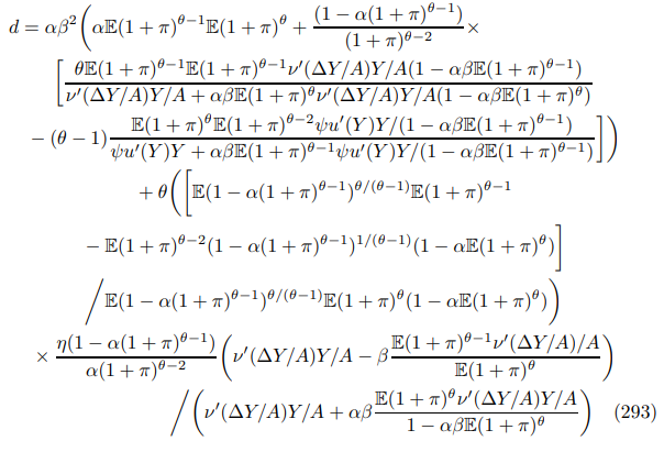
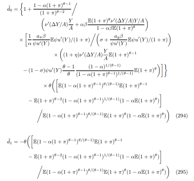
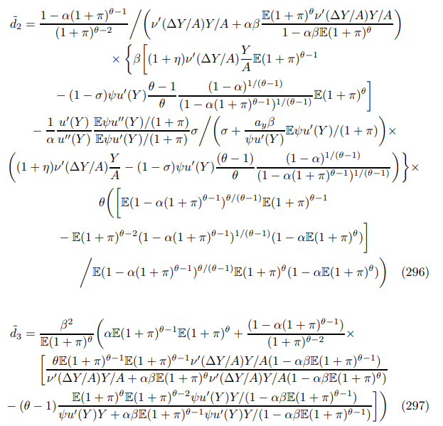
This subsection begins by gathering together the expression for the non-linear Phillips curve coefficients. The expressions are grouped into three subsubsections dealing in turn with the Phillips curve, the Euler and the price dispersion relation. The fourth covers the Phillips curve in the general small noise limit case. The final part solves for the singular surfaces around ZINSS.
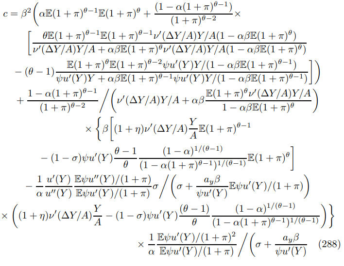
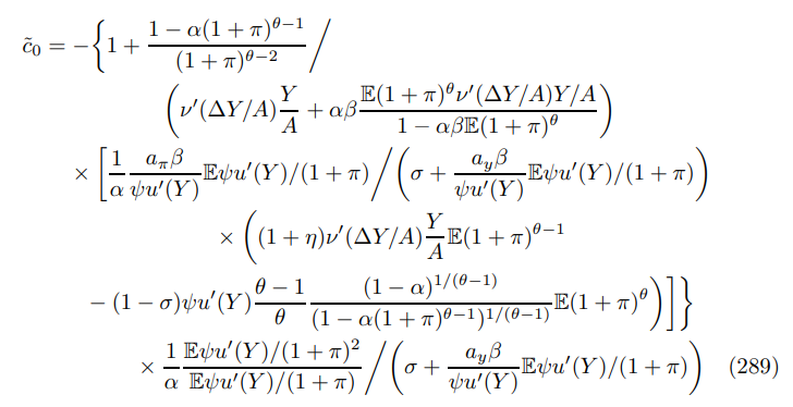
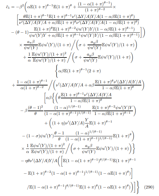
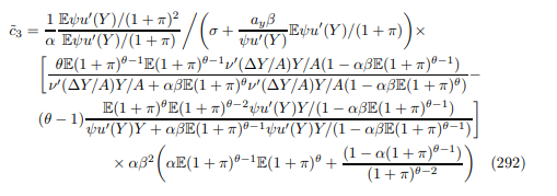
E.1.1 Phillips Curve (116)
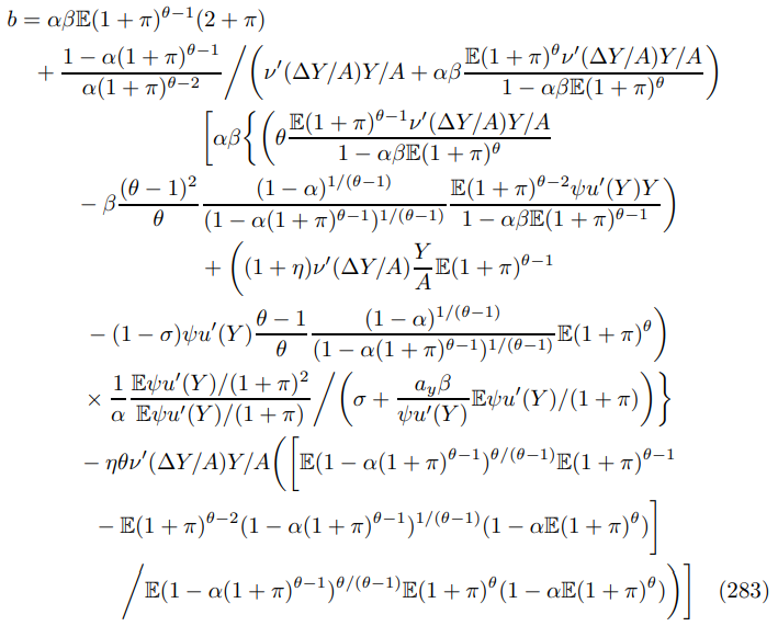
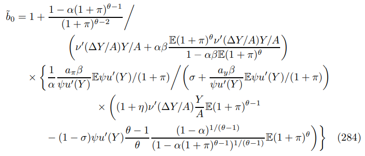
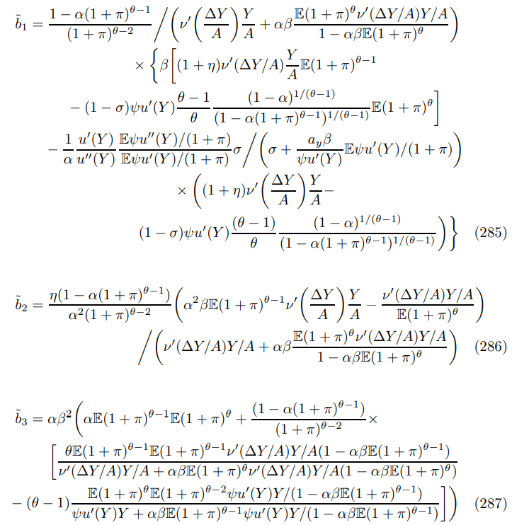
E.1.2 Euler Coefficients (117)

E.1.3 Price Dispersion
E.1.4 Trend Inflation Phillips Curve
This final part lays out the general Phillips curve in the small noise limit with arbitrary time preference and trend inflation. It compliments discussions of trend inflation and allows me to complete the proofs of Theorem 8 and Proposition 23. The justification of Footnote 92 is immediate.

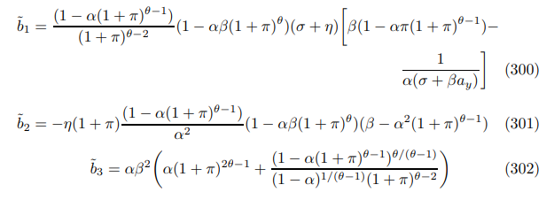
Remark 39. Symmetry arises in the error terms under trend inflation as under ZINSS. This reflects the inefficiency of aggregate fluctuations discovered in Theorem 6, which holds at any rate of trend inflation. However, it cannot be solved for without finding an exact form for the entire model which is beyond the perimeter of this study.
Remark 40. Symmetry breaks down in non-degenerate stochastic steady state, where non-vanishing uncertainty creates additional inter-temporal distortions, hence, the more complicated expressions in Section 6.2.
E.1.5 Singular Surfaces
This part completes the solution of the boundary surface. It justifies (5) and extends it to the |ε| limit, whilst generalizing it to the whole parameter space. Parametize the surface as follows

The bifurcated Phillips curve takes the form

where κ was defined back in (44). Substitute into the main Phillips curve (116) and suppressing the errors reveals

Substituting in the wall-crossing constraint from Proposition 20

Equating the coefficients between (302) with (304)


substituting in the primitives and splitting numerators from denominators, as before, yields
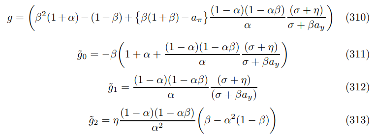
Finally, down the limit where β → 1 and σ = 1.
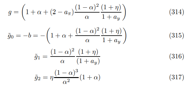
Note that these coefficients have clear predicted signs.
This paper is available on arxiv under CC 4.0 license.

