Author:
(1) David Staines.
Table of Links
4 Calvo Framework and 4.1 Household’s Problem
4.3 Household Equilibrium Conditions
4.5 Nominal Equilibrium Conditions
4.6 Real Equilibrium Conditions and 4.7 Shocks
5.2 Persistence and Policy Puzzles
6 Stochastic Equilibrium and 6.1 Ergodic Theory and Random Dynamical Systems
7 General Linearized Phillips Curve
8 Existence Results and 8.1 Main Results
9.2 Algebraic Aspects (I) Singularities and Covers
9.3 Algebraic Aspects (II) Homology
9.4 Algebraic Aspects (III) Schemes
9.5 Wider Economic Interpretations
10 Econometric and Theoretical Implications and 10.1 Identification and Trade-offs
10.4 Microeconomic Interpretation
Appendices
A Proof of Theorem 2 and A.1 Proof of Part (i)
B Proofs from Section 4 and B.1 Individual Product Demand (4.2)
B.2 Flexible Price Equilibrium and ZINSS (4.4)
B.4 Cost Minimization (4.6) and (10.4)
C Proofs from Section 5, and C.1 Puzzles, Policy and Persistence
D Stochastic Equilibrium and D.1 Non-Stochastic Equilibrium
D.2 Profits and Long-Run Growth
E Slopes and Eigenvalues and E.1 Slope Coefficients
E.4 Rouche’s Theorem Conditions
F Abstract Algebra and F.1 Homology Groups
F.4 Marginal Costs and Inflation
G Further Keynesian Models and G.1 Taylor Pricing
G.3 Unconventional Policy Settings
H Empirical Robustness and H.1 Parameter Selection
I Additional Evidence and I.1 Other Structural Parameters
I.3 Trend Inflation Volatility
D.2 Profits and Long-Run Growth
The first two subsubsections house the proofs of the two main propositions concerning long-run profits. The final subsubsection contains a final proof and fortifies empirical arguments concerning labour supply made in the profit section.
D.2.1 Proof of Proposition 13
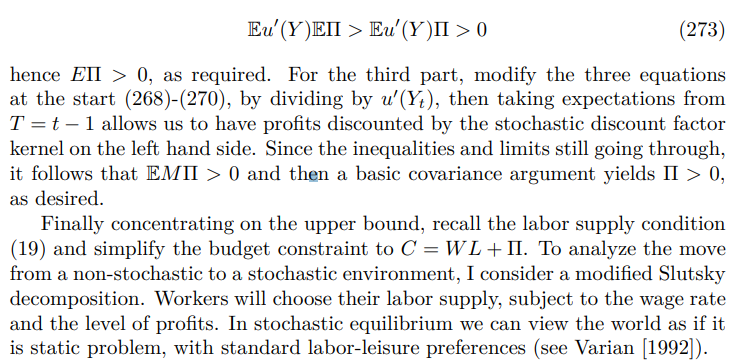
Proof. The proof starts with the lower bound where there are three cases and then finishes with the upper bound. For the lower bound the order of argument is (ii), (iii) then (i). Aggregate profit can be written as

where the subscript indicates the time since the last reset. Cross-multiplying, taking expectations and using the non-stochastic limit, to cancel out terms in the preference shock ψ from both sides, reveals that

in the patient limit; with the weight coming from the terms in (25) and the context of the resetting firms problem

because the demand curve slopes down and marginal costs are constant, we can see that


For Assumption 2 (iii), the proof comes from an analysis of covariance and (strict) stochastic monotonicity properties. By application of Theorem 1.A.3 and 1.A.8 of Shaked and Shanthikumar [2007] to the cases of above and below average profit, we know that the covariance

is strictly positive. Applying the definition of covariance.

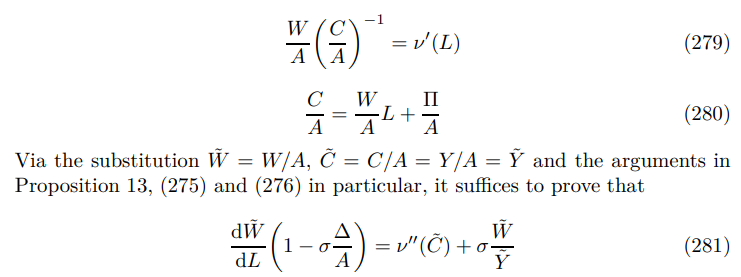
Therefore there will be three channels. A substitution effect from (lower) wages onto labor supply and two income effects, one from the change in wages and the other from the change in profits. Theorem 2 tells us that labor supply rises and wages fall. The strategy is to show that the first two effects net out to reduce labor supply. This means that profits must decrease, to generate a wealth effect that increases labor supply. To demonstrate this point, it is sufficient to show that the labor supply curve is positively sloped. Totally differentiating with respect to L

Simplifying yields

Since the right hand side is always positive, the sign of the derivative is determined by the bracket. Now substitute the production function in to create the determinant

D.2.2 Proof of Proposition 14

Proof. The result comes from a chain of inequalities. From the principle of optimality, it is clear that the firm is weakly better off when it can change prices. Furthermore, since we know that profit function is strictly concave, the optimization problem at any time will have a unique solution. Therefore, we can upgrade to strict inequalities

where I am using (25) (the profit function). Since the demand curve slopes down and there are no increasing returns to scale, we know that

D.2.3 Additional Arguments
The evidence on long-run labor supply elasticity is mixed. The consensus estimate appears to be zero associated with Doran [2014] and Berger et al. [2018], in which case the main result goes through. Ashenfelter et al. [2010] argues that the likely range is between -0.2 and 0.2 with their study at the lower range. The concern with unemployment and underemployment, in Mas and Pallais [2019], favours a positive figure. There is more discussion in the parametization Appendix I.

Proof. With balanced growth it has been established that σ = 1, whilst the labor supply and profit conditions take the form

and the proof will be complete if we can argue that the left hand bracket is strictly positive with probability one. To do so suppose the converse, then it follows from the definition of balanced growth in stochastic equilibrium that

This paper is available on arxiv under CC 4.0 license.

