Author:
(1) David Staines.
Table of Links
4 Calvo Framework and 4.1 Household’s Problem
4.3 Household Equilibrium Conditions
4.5 Nominal Equilibrium Conditions
4.6 Real Equilibrium Conditions and 4.7 Shocks
5.2 Persistence and Policy Puzzles
6 Stochastic Equilibrium and 6.1 Ergodic Theory and Random Dynamical Systems
7 General Linearized Phillips Curve
8 Existence Results and 8.1 Main Results
9.2 Algebraic Aspects (I) Singularities and Covers
9.3 Algebraic Aspects (II) Homology
9.4 Algebraic Aspects (III) Schemes
9.5 Wider Economic Interpretations
10 Econometric and Theoretical Implications and 10.1 Identification and Trade-offs
10.4 Microeconomic Interpretation
Appendices
A Proof of Theorem 2 and A.1 Proof of Part (i)
B Proofs from Section 4 and B.1 Individual Product Demand (4.2)
B.2 Flexible Price Equilibrium and ZINSS (4.4)
B.4 Cost Minimization (4.6) and (10.4)
C Proofs from Section 5, and C.1 Puzzles, Policy and Persistence
D Stochastic Equilibrium and D.1 Non-Stochastic Equilibrium
D.2 Profits and Long-Run Growth
E Slopes and Eigenvalues and E.1 Slope Coefficients
E.4 Rouche’s Theorem Conditions
F Abstract Algebra and F.1 Homology Groups
F.4 Marginal Costs and Inflation
G Further Keynesian Models and G.1 Taylor Pricing
G.3 Unconventional Policy Settings
H Empirical Robustness and H.1 Parameter Selection
I Additional Evidence and I.1 Other Structural Parameters
I.3 Trend Inflation Volatility
9.3 Algebraic Aspects (II) Homology
The first part introduces the theoretical building blocks. The second applies these constructs to the problem at hand. Appendix F.1 provides algebraic extensions and F.3 the dual theory.
9.3.1 Basic Homology and Cohomology Theory
Homological algebra studies holes in topological spaces. The original motivation was the observation that two shapes can be distinguished by examining their holes. For instance, a circle is not a disk because it has a hole whilst the disk is solid. Likewise, the ordinary sphere differs from a circle because it encloses a two rather than a one dimensional hole.
The building block of homology theory is called a cycle which forms a closed submanifold. They can be thought of as loops. For example, a line on a surface is a 1-cycle, a two dimensional surface like a disc cut out of a sphere is a 2 cycle. These cycles can be thought of as cuts or zippers that can be fastened or unfastened. A boundary is a cycle which is also the boundary of a submanifold. A homology class, which represents the hole or cut, is an equivalence class of cycles modulo boundaries. Therefore, a homology class is represented by a cycle which is not the boundary of any closed submanifold. Effectively, it is a "missing manifold". It is part of the space that would be added to form a Euclidean 1 cover. Here it represents economic effects and dynamic trade-offs, intrinsic to the model, that are absent from approximations taken from ZINSS.
The principle tool required is the homology group. The nth homology group represents behavior in dimension n. The 0th is called the fundamental group. It is trivial if the space is connected because every loop can be continuously deformed into a single point.[72] Appendix F.1 provides formal justification for these results.
The dual cohomology theory, expounded in F.3, explains how these holes are filled in. The main result here is once again De Rham’s theorem. It implies that holes are filled by singular surfaces with dimension equal to the difference between the ambient surface and the size of the hole. The intuition is that the only way that standard approximations of these models can break down is when a "rearrangement pattern" fails.
9.3.2 Application
Before proceeding to the bifurcation analysis around ZINSS, it is necessary to modify Theorem 6 to accommodate discounting.

Proof. The optimization of household welfare problem amounts to maximizing the real wage and therefore the real marginal costs, with respect to the choice of present inflation and its lag. The first order condition sets the marginal effect today to the discounted marginal wage loss tomorrow so
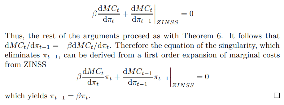
Appendix F.4 provides an elementary demonstration of the dynamic relationship between marginal costs and inflation.
The main application concerns the family of linear approximations at low volatility.

Proof. The proof follows swiftly from Proposition 8, the derivation of the two Phillips curves in 5.1, 7.1 and the calculations in E.1.4, which verify that none of the terms in the Phillips curve drop out, when we fix β < 1.
Remark 22. The same construction would work for a sequence of approximations at different rates of trend inflation. There would be no problem if I considered the √ ε case because the ramification of this cover in a single variable does not generate a hole.

This motivates the limiting concept and indeed the entire stochastic equilibrium concept from an a priori New Keynesian standpoint.
The following decomposition, derived from (112), serves to locate the components of the singularity and justifies the claims for the √ ε limit case made at the start. It starts by moving all the terms to the left hand side.
Decomposition 1.
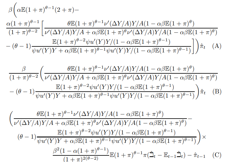
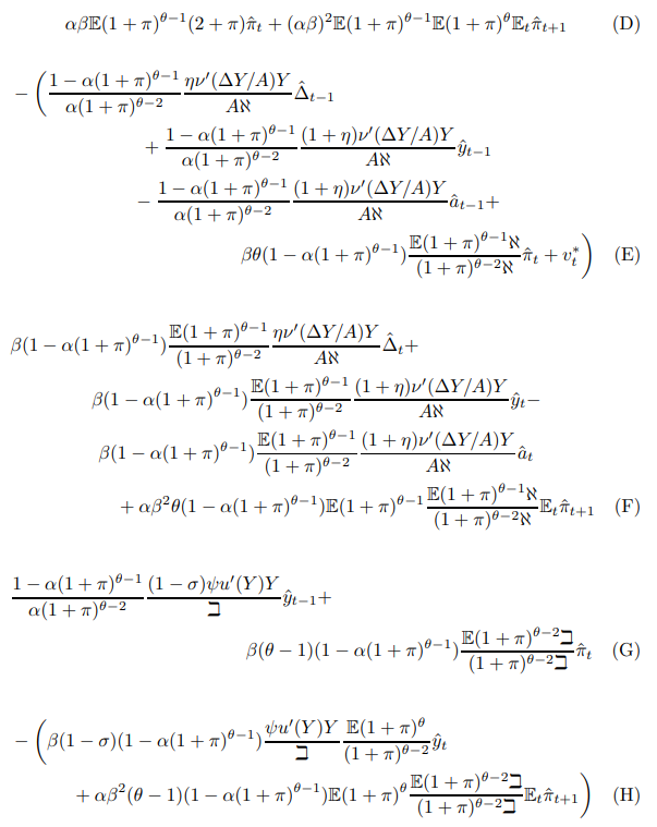
The relation with the equations in Section 2 is as follows:
i (A) + (F)+(H) = 0 ≡ (1)
ii (B) + (C) = 0 ≡ (3)
iii (D) + (E) + (G) = 0 ≡ (5)
The De Rham cohomology allows me to integrate each of these collections of terms to form surfaces. It is therefore clear that the homology / cohomology would extend to higher order approximations, as this would simply improve the approximation of each singular surface. Geometrically, the sum of all the terms represents the ambient space, whilst (ii), (iii) are holes that glue together to form a singular surface enclosing (i). The demand side disturbance term, which vanishes at ZINSS, reflects interactions between the shocks and output terms, uncovered back in Proposition 10.
The second surface (ii) represents the constraint that prices today equal prices tomorrow. This follows thanks to Proposition 1 that maps between reset prices and inflation. This step arises out of the non-cancellation of the lag operators in (108) and (109). It is therefore necessary to the whole bifurcation, representing the wall of the crossing between the two Phillips curves. It is now clear why dynamics on surface (i) are entirely forward-looking once re-optimization constraints have been removed. It is sub-optimal for firms to condition on past events, as it would be for the policymaker, which is made clear in Proposition 9. The error term here represents intertemporal distortions caused by stochasticity. It is of order π around ZINSS and therefore vanishes to leave a non-stochastic limiting relationship.
The third surface is the "residual" surface. It arises automatically from the need to use the lagged Euler (114) to substitute out lagged output. It cleanses the model of inter-temporal forces. In an exactly determined system it is not a problem if one of the surfaces is less intuitive; if the system has N dimensions then there are N − 1 degrees of freedom and the last adjusts to equilibriate the model. This confirms that it represents General Equilibrium Effects. The expression for the approximation around ZINSS is housed in Appendix E.1.
Returning to our prime approximation, the salient point is that ZINSS is the site of a "hole within a hole". Throughout the state space there is a two-dimensional hole with codimension one. This reflects the fact that reoptimization constraints necessarily induce a cost channel and an inter-temporal substitution motive. At ZINSS, in the first order expansion, there is an additional singularity "inside" the ambient singular surface given by (4). This acts to destroy the present shock term coming from the demand side necessitated by their cancellation from the other singular components. Elsewhere, this constraint drops out because in general there will be a value of inflation for which re-optimization constraints break down, even though there is a non-equilibrium realization of the main shock. We can always view the second constraint (5) as acting to remove this lagged error term, in the way that the first constraint (3) is removing lagged inflation.
If the approximation is such that a supply shock enters, there must be another component of the singular surface to eliminate it. In general, surface (5) scales with the number of variables that are used to flesh out the economy’s neoclassical skeleton. Therefore, this bifurcation analysis extends to the medium and large models used at central banks. The formalization is as follows:
Proposition 22. The homology of the various versions of the non-linear Calvo Phillips curve are
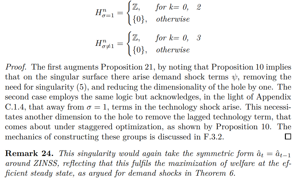
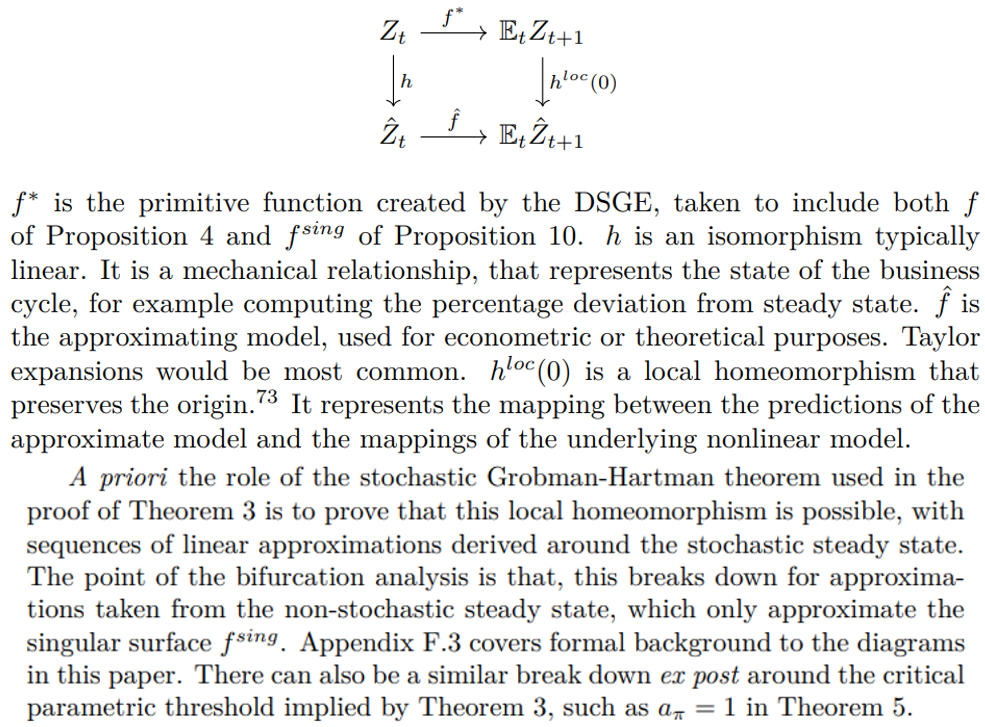
The following diagram offers insights into both the strands of bifurcation analysis throughout the paper
Figure 1: Well-Behaved Approximations
This paper is available on arxiv under CC 4.0 license.

[73] The focus on local homeomorphism is motivated by the application of perturbation techniques. It would be too demanding to seek global relationships. After all, economists do not expect an approximation to be globally accurate.

