Author:
(1) David Staines.
Table of Links
4 Calvo Framework and 4.1 Household’s Problem
4.3 Household Equilibrium Conditions
4.5 Nominal Equilibrium Conditions
4.6 Real Equilibrium Conditions and 4.7 Shocks
5.2 Persistence and Policy Puzzles
6 Stochastic Equilibrium and 6.1 Ergodic Theory and Random Dynamical Systems
7 General Linearized Phillips Curve
8 Existence Results and 8.1 Main Results
9.2 Algebraic Aspects (I) Singularities and Covers
9.3 Algebraic Aspects (II) Homology
9.4 Algebraic Aspects (III) Schemes
9.5 Wider Economic Interpretations
10 Econometric and Theoretical Implications and 10.1 Identification and Trade-offs
10.4 Microeconomic Interpretation
Appendices
A Proof of Theorem 2 and A.1 Proof of Part (i)
B Proofs from Section 4 and B.1 Individual Product Demand (4.2)
B.2 Flexible Price Equilibrium and ZINSS (4.4)
B.4 Cost Minimization (4.6) and (10.4)
C Proofs from Section 5, and C.1 Puzzles, Policy and Persistence
D Stochastic Equilibrium and D.1 Non-Stochastic Equilibrium
D.2 Profits and Long-Run Growth
E Slopes and Eigenvalues and E.1 Slope Coefficients
E.4 Rouche’s Theorem Conditions
F Abstract Algebra and F.1 Homology Groups
F.4 Marginal Costs and Inflation
G Further Keynesian Models and G.1 Taylor Pricing
G.3 Unconventional Policy Settings
H Empirical Robustness and H.1 Parameter Selection
I Additional Evidence and I.1 Other Structural Parameters
I.3 Trend Inflation Volatility
8 Existence Results
This section is divided into three subsections: the first sets out the mathematical results central to the entire paper. The second introduces a concept key to the proof and then proves two major theorems. The third offers general discussion.
8.1 Main Results
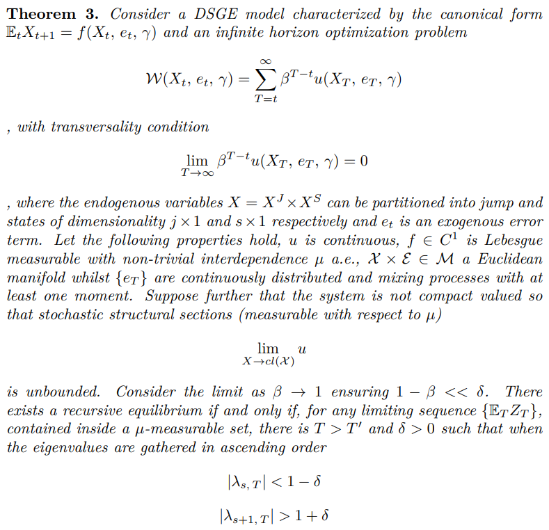
The first two theorems consist of existence and uniqueness results, for the main equilibrium concept here in the model, with appropriate generalization to a wider class of DSGE models.
8.1.1 Main Theorems
This part sets out the main theorems and discusses some of the primitive assumptions.

Remark 10. Non-trivial interdependence rules out systems where one or more endogenous variables actually evolve independently, such that diagonalization will not work to reassign eigenvalues. It formalizes intuitive understanding of the difference between endogenous and exogenous variables.

Remark 12. The stochastic section idea is important to rule out boundaries that are reached with zero probability because they require precise configurations among the exogenous shocks. From a topological standpoint, this allows me to avoid considering pieces at the boundary of an open m dimensional manifold that are not regular, in the sense of being m − 1 dimensional.[58] This point will prove useful in application.
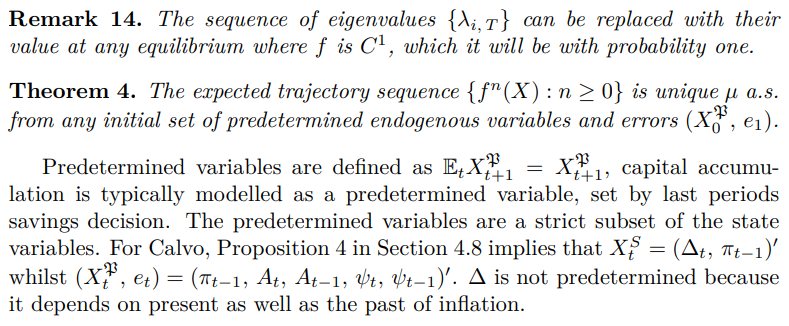
Remark 13. The eigenvalue condition is necessary and sufficient for a stochastic equilibrium (ergodic invariant measure) for the recursive equilibrium of X, even if there is no transversality or infinite horizon optimization condition. The other conditions are used to generate necessity of stochastic equilibrium.

Remark 15. An expected trajectory corresponds with the loose conception of recursive equilibrium prevailing in the previous New Keynesian literature. The theorem justifies the association of f with recursive equilibrium and clarifies that Classical and New Keynesian notions are in fact equivalent. It definitively demonstrates that indeterminacy is not in fact a standard feature of DSGE.
8.1.2 Application
This part confirms that the theorems apply to the two main models here. It also discusses some models which are not covered and completes the analysis for Rotemberg.
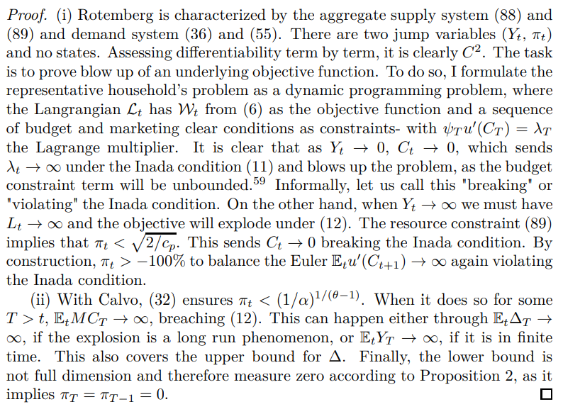
Proposition 16. Both Calvo and Rotemberg models meet the primitive conditions to apply Theorem 3.
The proof is split into two points starting with Rotemberg.

Remark 16. If σ = 1 we could just consider the objective function W and not worry about the dynamic programming problem for the Rotemberg component.
Remark 17. In both cases the relevant objective function diverges to −∞, so the result is not a figment of measurability restrictions. The problem with indeterminacy is that it is based on conditional convergence of one or more forward solution variables in the linear approximation. However, with the underlying non-linear system there is divergence.
Remark 18. There are models that do not meet the boundary explosion condition. This includes menu costs and similar models, where there is a fixed cost of adjustment (see Stokey [1989], and Stokey [2009]).[60] In the standard menu cost model if inflation is high enough all firms will choose to pay it and a flexible price system will arise. The suggestion is that the various compactness assumptions used elsewhere in the general equilibrium and mean field game literatures to prove unconditional existence (not depending on parameters or shock distributions) are necessary in a broad class of models.
Remark 19. Dropping the boundary conditions can also represent a threat to uniqueness. Consider the canonical overlapping generations model of Samuelson [1958] and its many subsequent extensions, where multiple asset bubble equilibria can develop from intrinsically valueless assets.
I can proceed immediately to analyzing Rotemberg.

Proof. Follows immediately from Proposition 16 (i), Corollary 1, Proposition 8 and Theorem 3.
For Calvo the best general result is
Proposition 17. There exists a recursive equilibrium if in the limit as β → 1 the following inequality holds

Proof. Proposition 16 (i), Proposition 4 and Theorem 3 serve to demonstrate that there have to be two roots inside and two roots outside the unit circle. The final result comes from applying the bound of Rouche’s theorem[61] (for precisely two roots outside the unit circle) to the eigenvalue polynomial derived in Appendix E.3 and displayed later as (167).
This condition is not necessary for a solution. Bounds are often far from sharp and could be economically uninformative. Alternatively, there is a rather unwieldy quartic formula, which can be found in Auckly [2007], that would yield necessary conditions. Appendix E.4.4 extends the analysis to the case with no price dispersion and looks at conditions that imply non-existence. The idea could naturally be applied across a wide range of DSGE. It could potentially be used alongside the techniques in Theorem 2 and developments thereof to analyze the function space of shocks that support equilibrium. This would take us outside the scope of an economics journal.
This paper is available on arxiv under CC 4.0 license.
[58] Unfamiliar readers may wish to consult a text like Munkres [2018].
[59] This is because lifetime income will be strictly bigger than zero. Technically with Calvo, I will be calling in Proposition 13 to ensure losses do not swallow household’s labor income. If this happened the blow-up would be automatic.
[60] This is also true in classical models where there is some outside option, for example a firm could exit the industry at no cost or the household could subsist from social security benefits.
[61] This is a standard result in complex analysis, consult Stein and Shakarchi [2010].

