Author:
(1) David Staines.
Table of Links
4 Calvo Framework and 4.1 Household’s Problem
4.3 Household Equilibrium Conditions
4.5 Nominal Equilibrium Conditions
4.6 Real Equilibrium Conditions and 4.7 Shocks
5.2 Persistence and Policy Puzzles
6 Stochastic Equilibrium and 6.1 Ergodic Theory and Random Dynamical Systems
7 General Linearized Phillips Curve
8 Existence Results and 8.1 Main Results
9.2 Algebraic Aspects (I) Singularities and Covers
9.3 Algebraic Aspects (II) Homology
9.4 Algebraic Aspects (III) Schemes
9.5 Wider Economic Interpretations
10 Econometric and Theoretical Implications and 10.1 Identification and Trade-offs
10.4 Microeconomic Interpretation
Appendices
A Proof of Theorem 2 and A.1 Proof of Part (i)
B Proofs from Section 4 and B.1 Individual Product Demand (4.2)
B.2 Flexible Price Equilibrium and ZINSS (4.4)
B.4 Cost Minimization (4.6) and (10.4)
C Proofs from Section 5, and C.1 Puzzles, Policy and Persistence
D Stochastic Equilibrium and D.1 Non-Stochastic Equilibrium
D.2 Profits and Long-Run Growth
E Slopes and Eigenvalues and E.1 Slope Coefficients
E.4 Rouche’s Theorem Conditions
F Abstract Algebra and F.1 Homology Groups
F.4 Marginal Costs and Inflation
G Further Keynesian Models and G.1 Taylor Pricing
G.3 Unconventional Policy Settings
H Empirical Robustness and H.1 Parameter Selection
I Additional Evidence and I.1 Other Structural Parameters
I.3 Trend Inflation Volatility
8.2 Key Proofs
This part has three subdivisions. The first covers analytic prerequisites, the second proves Theorem 3, the main effort of this paper, whilst the third proves Theorem 4.
8.2.1 Compactness
Before the proofs appear, it is necessary to introduce the key compactness property. First, a preliminary definition is needed. It prevents the probability measure "escaping to infinity".

It has been widely applied in econometrics and microeconomics. The compactness property specializes tightness to expected paths.

The proof has four strands. The first uses compactness and continuity to prove that stochastic equilibrium is necessary. The second demonstrates the desired eigenvalue configuration is consistent. The third uses a bounding by a suitable linear function to demonstrate that alternative configurations are not consistent with stochastic equilibrium. Finally, a suitable smoothness argument is used to rule out some pathological cases.
8.2.2 Proof of Theorem 3
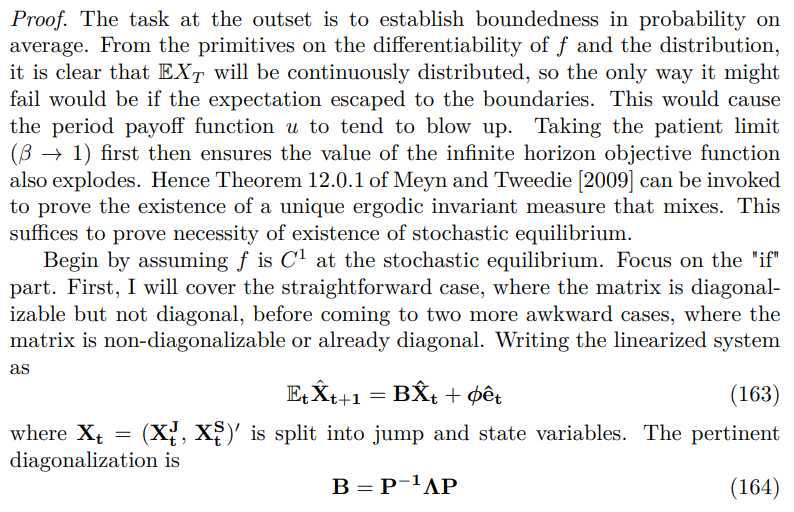
where Λ contains all the eigenvalues λi along its diagonal and zeros elsewhere. This Jordan decomposition is not unique, in particular the eigenvalues can be reordered as desired.[62] The convenient form is to block by ascending order so
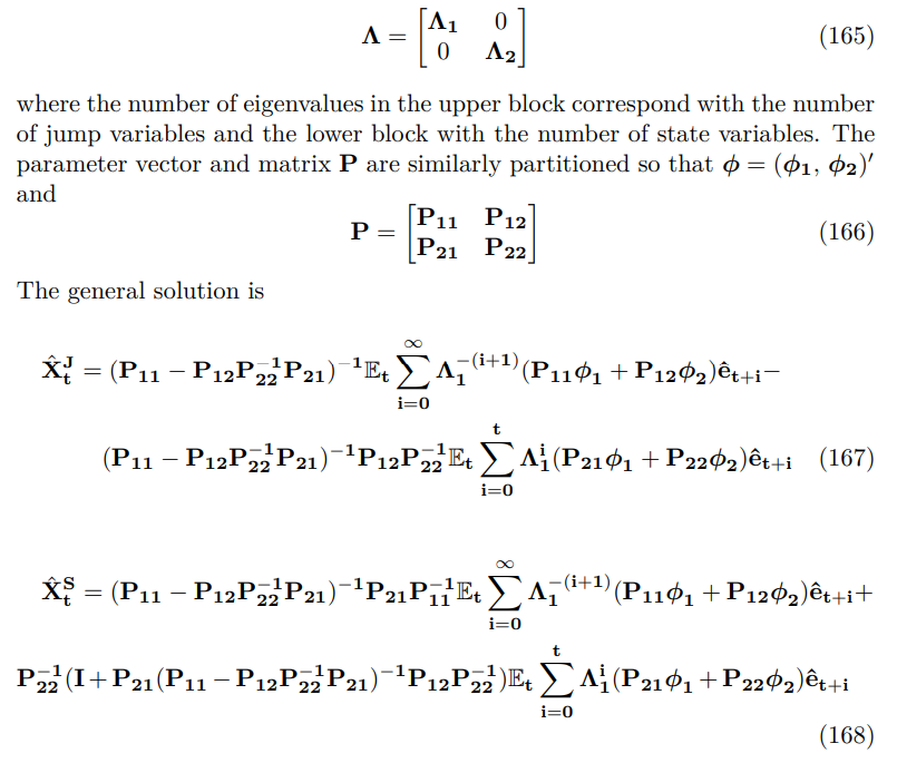
Appendix E.3 breaks down the linear algebra. This part of the proof is completed by verifying that the infinite horizon dynamical system, implied by the spectral decomposition, is consistent with stochastic equilibrium. The decomposition yields
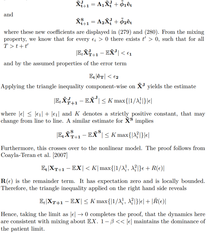
There are three special cases: first where the matrix is already diagonal, second where it cannot be diagonalized and third where inverse matrices used in the solution (167) and (168) do not exist. In all instances these problems function as removable singularities (because of the primitives on f) that can be treated by considering suitable perturbations.
Let us start with the case where the matrix is already diagonal, where we cannot permute the eigenvalues. Clearly, this can only arise when all the off diagonal elements are zero. Local non-trivial dependence and Lebesgue measurability ensure this is a zero-probability event that can be ignored in stochastic equilibrium.
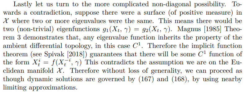
The next steps of the proof treat the reverse implication, by ruling out alternative eigenvalue configurations. I proceed by contradiction, starting with instances where there are more or fewer eigenvalues inside the unit circle than jump variables but no eigenvalues on the unit circle, before finishing with these knife-edge cases. The previous arguments have established that around any candidate stochastic equilibrium

When there are too few eigenvalues in the unit circle, the system will blow up (EX∗ → ∞ for any |ǫ| > 0) under the influence of an inverse eigenvalue lying outside the unit circle from the first block. With too many the result will be the same but the culprit will be an eigenvalue from the second block.
The final configuration to consider is where there are eigenvalues on the unit circle. I cannot use the Grobman-Hartman theorem, but we can use the geometric properties of stochastic equilibrium. By the continuity properties of f and its eigenvalues (Rahman and Schmeisser [2002]), we can see that any equilibrium with eigenvalues on the unit circle would have to be arbitrarily close to one where the number of jump variables and eigenvalues outside the unit circle do not match up. Likewise, the objective function would also have to be arbitrarily close to its values in these equilibria but this is impossible since we have already shown that the objective function u diverges in these cases.[63]

8.2.3 Proof of Theorem 4
Proof. Towards a contradiction, note that if there were multiple trajectories stemming from the same combination of predetermined and state variables then there would exist two function
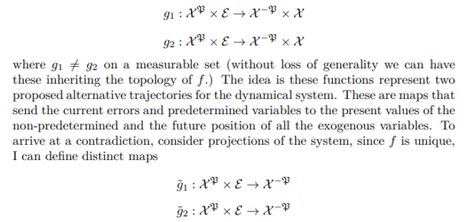
Now take expectations with respect to the ergodic measure, if there is no measurable set Ω such that

take a subsection

since the two maps are probabilistic and distinct, by assumption, it must be the case that for some Ω

This violates Birkhoff’s ergodic theorem (Theorem 1). We have reached a contradiction.
This paper is available on arxiv under CC 4.0 license.
[62] All the matrix algebra here is contained in Abadir and Magnus [2005] or any good undergraduate linear algebra text.
[63] The dominance of the patient limit is crucial because the blow-up of the linearized system would be non-uniform in β because no β < 1 could rule out eigenvalues on the unit circle.

