Author:
(1) David Staines.
Table of Links
4 Calvo Framework and 4.1 Household’s Problem
4.3 Household Equilibrium Conditions
4.5 Nominal Equilibrium Conditions
4.6 Real Equilibrium Conditions and 4.7 Shocks
5.2 Persistence and Policy Puzzles
6 Stochastic Equilibrium and 6.1 Ergodic Theory and Random Dynamical Systems
7 General Linearized Phillips Curve
8 Existence Results and 8.1 Main Results
9.2 Algebraic Aspects (I) Singularities and Covers
9.3 Algebraic Aspects (II) Homology
9.4 Algebraic Aspects (III) Schemes
9.5 Wider Economic Interpretations
10 Econometric and Theoretical Implications and 10.1 Identification and Trade-offs
10.4 Microeconomic Interpretation
Appendices
A Proof of Theorem 2 and A.1 Proof of Part (i)
B Proofs from Section 4 and B.1 Individual Product Demand (4.2)
B.2 Flexible Price Equilibrium and ZINSS (4.4)
B.4 Cost Minimization (4.6) and (10.4)
C Proofs from Section 5, and C.1 Puzzles, Policy and Persistence
D Stochastic Equilibrium and D.1 Non-Stochastic Equilibrium
D.2 Profits and Long-Run Growth
E Slopes and Eigenvalues and E.1 Slope Coefficients
E.4 Rouche’s Theorem Conditions
F Abstract Algebra and F.1 Homology Groups
F.4 Marginal Costs and Inflation
G Further Keynesian Models and G.1 Taylor Pricing
G.3 Unconventional Policy Settings
H Empirical Robustness and H.1 Parameter Selection
I Additional Evidence and I.1 Other Structural Parameters
I.3 Trend Inflation Volatility
D Stochastic Equilibrium
This section aligns with Section 6 of the main text. It begins by setting out the non-stochastic equilibrium conditions, before moving onto to the three omitted proofs and addressing the claims made in Remark 8.
D.1 Non-Stochastic Equilibrium
This subsection divided in two the first part details the closed form of the solution in terms of primitive parameters. The second explains why we must restrict the model to allow for economic growth and de-trending.
D.1.1 Exact Form
With functional forms in, the non-stochastic steady state is as follows

where I have used the price-setting relation. Therefore, thanks to constant returns the wage rate is

Price dispersion is

Inverting the marginal cost function and substituting in the price dispersion relationship yields

The resource constraint yields the solution for labor supply

The aggregate profit rate is

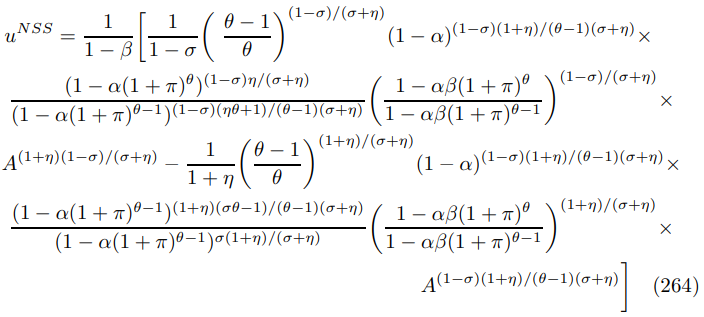
substituting into the utility function reveals that

Finally, present discounted welfare is

In line with the discussion in the text about profitability with trend inflation, firms will make different profits depending on when they last reset their price. Denoting the time since the last reset by the age of its price a

D.1.2 Economic Growth and De-trending
It is useful to examine the consequences of allowing for economic growth. To do so suppose there is exogenous technological progress at rate g so

To justify the practice of linear de-trending standard in empirical work, a balanced growth path is required. However, the following result demonstrates that this necessitates a specific parametric restriction.
Proposition 29. There exists a balanced growth path if and only if σ = 1.
Proof. There can be a balanced growth path if and only if we can solve for detrended output Y/A that does not depend on the growing variable A. Repeating the steps used to derive the steady state with no growth reveals that

where k is a function of only the behavioural parameters that could be calculated directly from (261). It is clear independence only arises when the exponent is zero which corresponds to σ = 1.
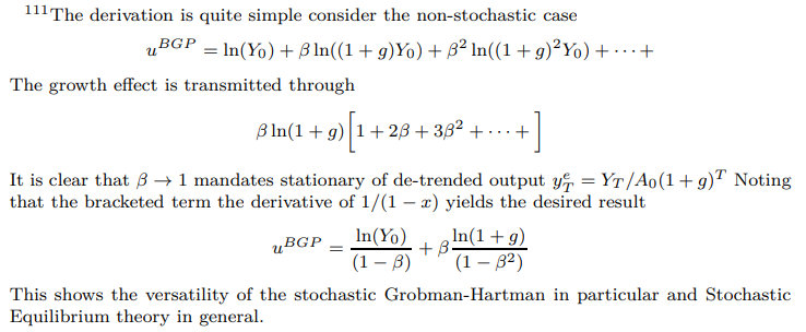
Therefore, I select σ = 1 for quantitative work here, since I am working with small noise limits and desire consistency with standard econometric practice. Although, this value is not ubiquitous in the literature, in the calibration section I demonstrate that it is consistent with a body of empirical evidence and prior work. In fact, Theorem 3 and all the subsequent analysis would go through in this case. Expected utility on the balanced growth path (BGP) would be augmented by a term reflecting the value of future growth. [111] Adding capital would avoid this knife-edge condition, at the expense of complicating the rest of the analysis.
This paper is available on arxiv under CC 4.0 license.


