Andrea Renzetti, Department of Economics, Alma Mater Studiorium Universit`a di Bologna, Piazza Scaravilli 2, 40126 Bologna, Italy.
Table of Links
Forecasting with the TC-TVP-VAR
Response analysis at the ZLB with the TC-TVP-VAR
A Appendix
A.1 Theory Coherent TVP-VAR
A.1.1 Time Varying Parameters by dummy observations
Starting from:

we can write the TVP-VAR in static compact form as:

Suppose we want to specify independent RW stochastic processes for all the coefficients in Φ as:
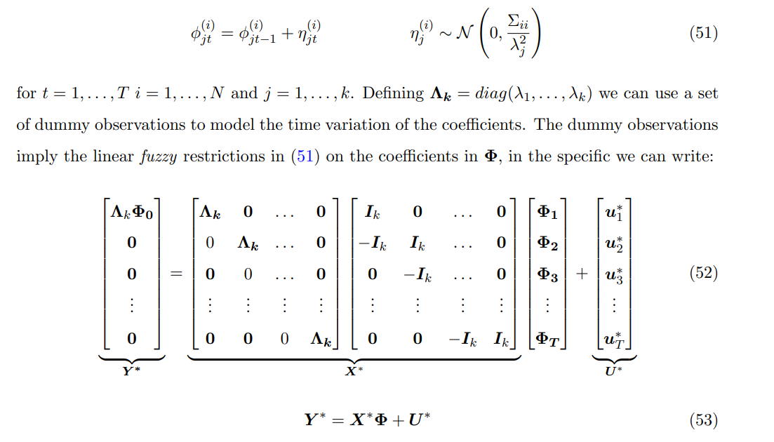
This is just another way of writing:
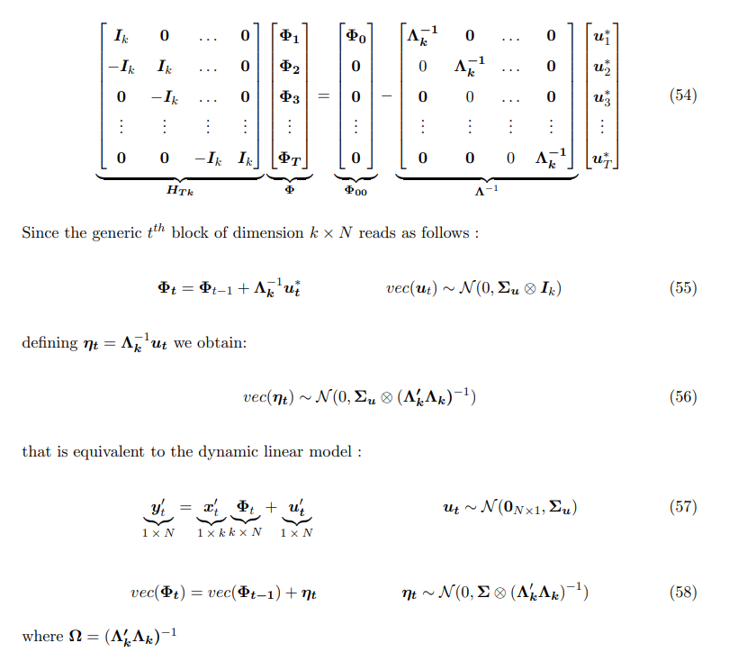
A.1.2 Population moments

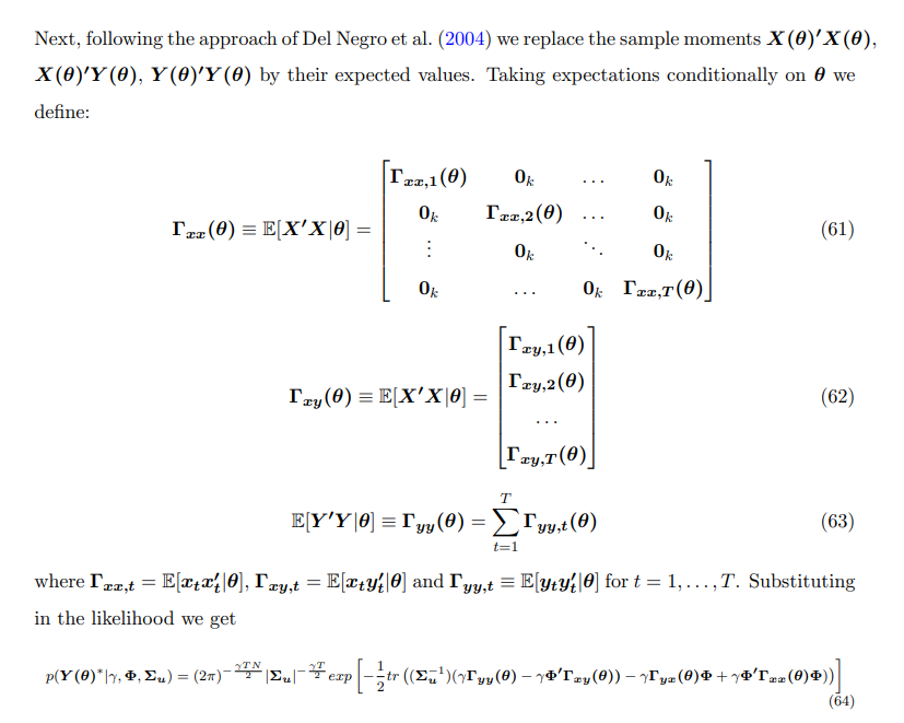
A.1.3 Integrating constant of the theory coherent prior
The integrating constant of the Normal-Inverse-Wishart prior

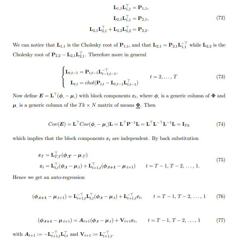
A.1.4 Conditional distribution of theory coherent prior
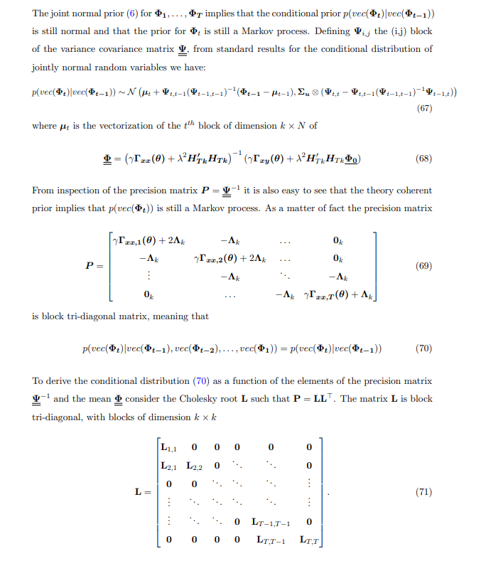
Considering the three first blocks we get
A.1.5 Marginal likelihood and fit-complexity trade off
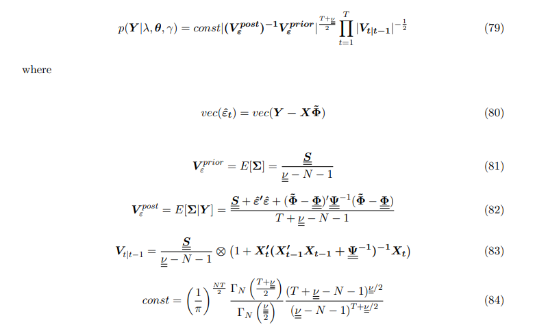
The marginal likelihood is given by:

Following the same steps as in (Giannone et al. 2015) it can be re-written as :
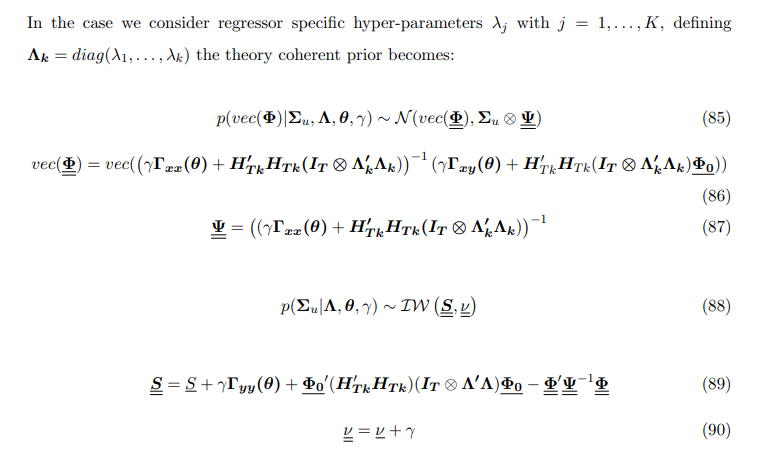
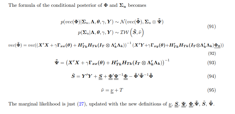
A.1.6 Formulas with distinct λj for j = 1, . . . ,K
A.2 Small scale New Keynesian model for the forecasting exercise
A.2.1 Data

A.2.2 Competing models in the forecasting exercise
The competing models in the out of sample forecasting exercise in Section 3 are
• A constant parameters VAR with flat prior.
• A constant parameters VAR with Normal Inverse-Wishart prior.
• A TVP-VAR model
The VAR with Normal Inverse-Wishart prior is given by:

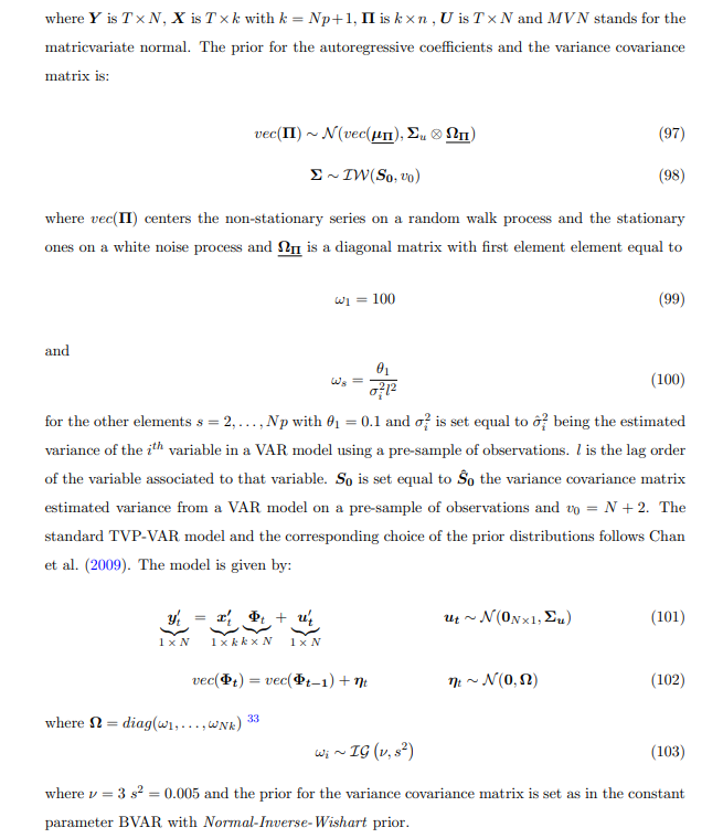
A.2.3 Prior for the DSGE parameters
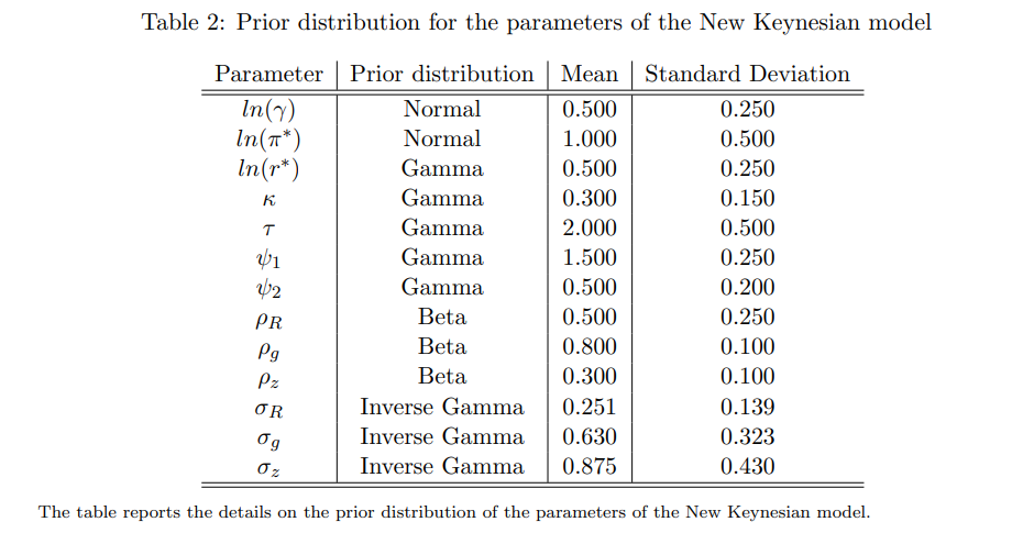
A.2.4 Posterior estimate for the DSGE parameters and IRFs from the TC-TVPVAR
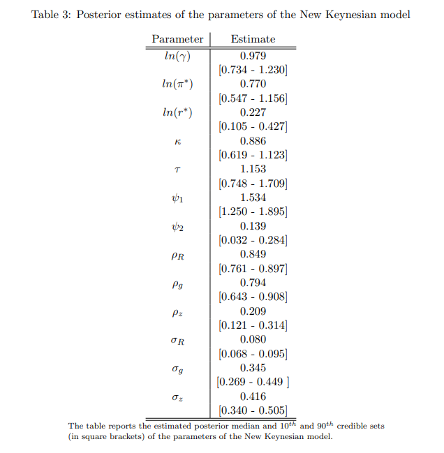
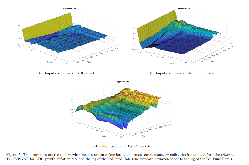
A.3 Medium scale New Keynesian model
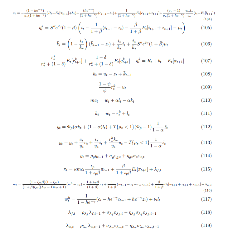
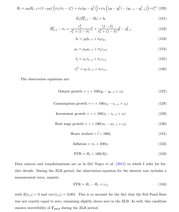
The model is taken from Del Negro et al. (2015) and it is a version of the popular medium scale New Keynesian model in Smets et al. (2007). The set of log-linearized equilibrium conditions of the model is
This paper is available on arxiv under CC 4.0 license.


