Authors:
(1) Matthew Sprintson
(2) Edward Oughton
Table of Links
2. Literature Review
2.1 Reviewing Broadband Infrastructure’s Impact on the Economy
2.2 Previous Research into IO Modeling of Broadband Investment
2.3 Context of the Bipartisan Infrastructure Act through Previous Research
3. Methods and 3.1 Leontief Input-Output (IO) Modeling
3.2 Ghosh Supply-Side Assessment Methods for Infrastructure
4.2 What are the GDP impacts of the three funding programs within the Bipartisan Infrastructure Law?
5. Discussion
5.2 What are the GDP impacts of the three funding programs within the Bipartisan Infrastructure Law?
5.3 How are supply chain linkages affected by allocations from the Bipartisan Infrastructure Law?"
Acknowledgements and References
3 Methods
In this section, various macroeconomic methods for assessing the contribution of infrastructure to the economy will be assessed. We begin by articulating a general macroeconomic system model based on IO, before detailing different demand-side and supply-side evaluation methods for broadband infrastructure.
3.1 Leontief Input-Output (IO) Modeling
The IO approach begins by dividing the economy into n sectors, such as agriculture, manufacturing, energy, telecommunications, and other such industries. The model denotes inter-sectoral transfers as zij , representing the dollar value of transfers from sector i to sector j. For example, if sector 1 is electricity and sector 2 is telecommunications, z12 represents the dollar value of electricity sold to the telecommunications industry as an input. The other metric is fi , which denotes the final demand for the good or service from sector i. The final demand includes purchases by consumers, investments from businesses, purchases from the government, and net exports.
The final output of sector i is denoted as xi , measured here in dollars, and represents the sum of all monetary values of the transactions from other inter-industry sectors, as well as the final demand for goods or services, stated in equation (1) as follows.

Thus, we can list the linear equations of all n industries in rows, as detailed in equation (2).

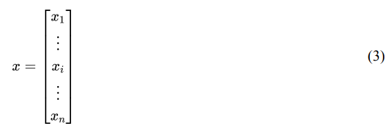
Moreover, the vector for the final output is x, as outlined in equation (3).

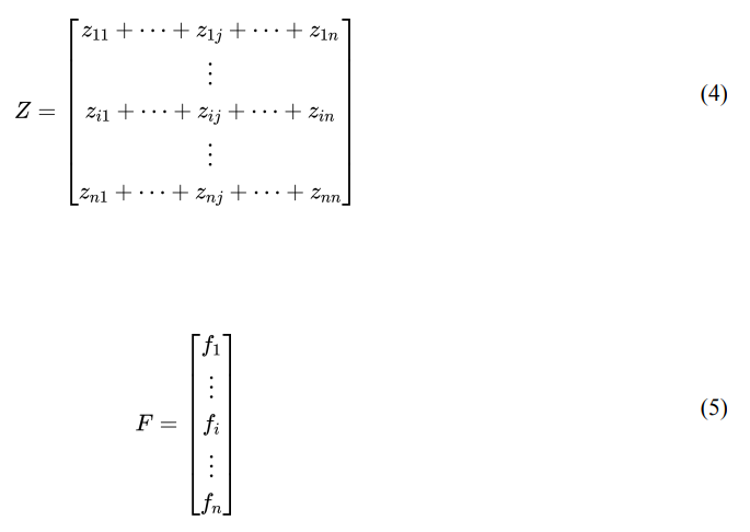
Likewise, the matrix of inter-industry transactions and final demand can be represented as Z and F, respectively, as we present in equations (4) and (5).

As each sector of the economy can be modeled in a row of the matrices above, the total expression for the total n industries in the economy can be modeled in a system of linear equations represented in equation (6).

Where i represents an identity matrix of dimensions n by n.
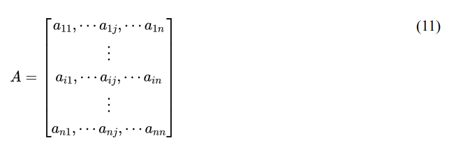
Each row of the matrix Z represents the aggregate output of its respective sector. To measure spillovers across industries, we can analyze technical coefficients aij = zij /xj . For two industries i and j, the technical coefficient aij is equal to the dollar's worth of input from i to the output of sector j.
Because zij = aij * xj , we can replace the respective coefficients algebraically, as detailed in equation (7).

Distributing, as per equation (8).

Factoring, as per equation (9).

Thus, as per the system of linear equations (10).

Where A is the n by n matrix of technical coefficients as represented below, in equation (11).

And the inverse of (I-A) is denoted as L, the Leontief-inverse matrix, as per equation (12

Therefore, we can use this formula to quantify the output generated by a shift in final demand for individual industrial sectors, or the whole economy.
This paper is available on arxiv under CC0 1.0 DEED license.

